Chapter - Communicating with Visualization
Supplementary chapter prepared for the BWXT Data Science Workforce Training Pilot. This material is original to the program.
About this chapter
Making a chart for yourself while exploring data is one thing; making a chart that communicates to a stakeholder is another. The competency map lists reporting and visualization as a named skill. This chapter covers the principles of charts that inform and persuade — the difference between a plot that you understand and one that anyone can.
A chart has a job
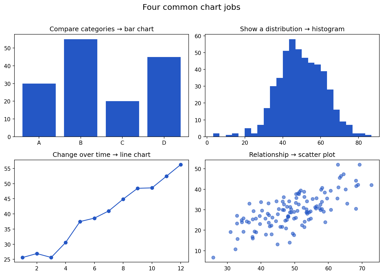
Before choosing a chart type, decide what question it answers. Most charts do one of four jobs:
| Job | Good chart |
|---|---|
| Compare values across categories | bar chart |
| Show a distribution | histogram, box plot |
| Show change over time | line chart |
| Show a relationship between two numbers | scatter plot |
If you cannot say in one sentence what a chart shows, it is not ready.
Show the code that generated this plot
import numpy as np
import matplotlib.pyplot as plt

rng = np.random.default_rng(0)
fig, axes = plt.subplots(2, 2, figsize=(10, 7))

axes[0, 0].bar(['A', 'B', 'C', 'D'], [30, 55, 20, 45], color='#2457c5')
axes[0, 0].set_title('Compare categories -> bar chart')

axes[0, 1].hist(rng.normal(50, 12, 500), bins=25, color='#2457c5')
axes[0, 1].set_title('Show a distribution -> histogram')

months = np.arange(1, 13)
axes[1, 0].plot(months, 20 + 3 * months + rng.normal(0, 2, 12), marker='o', color='#2457c5')
axes[1, 0].set_title('Change over time -> line chart')

x = rng.normal(50, 10, 120)
axes[1, 1].scatter(x, 0.6 * x + rng.normal(0, 6, 120), color='#2457c5', alpha=0.6)
axes[1, 1].set_title('Relationship -> scatter plot')
plt.tight_layout()
plt.show()
Principles for charts that communicate
- One message per chart. Decide the single takeaway and make it obvious.
- Label directly. Title, axes, and units. A reader should understand it without you in the room.
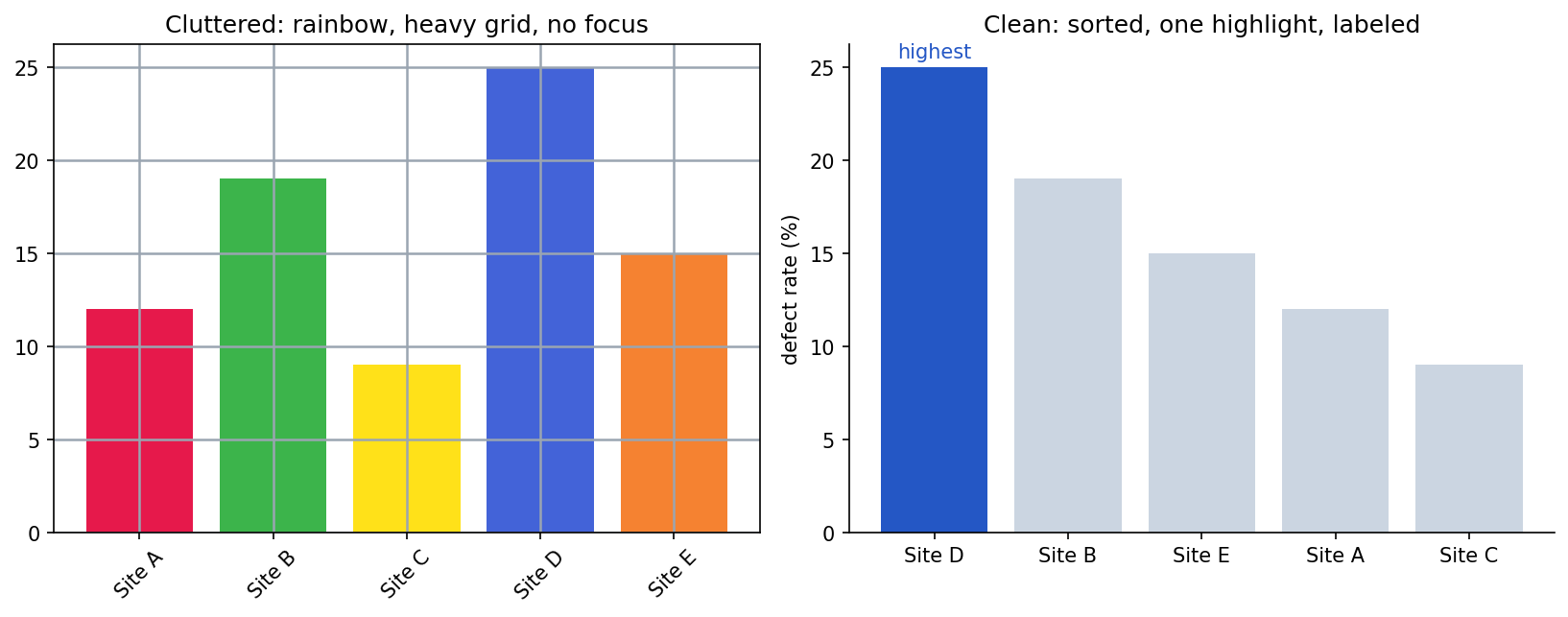
- Remove clutter. Drop gridlines, 3D effects, and decoration that do not carry information.
- Order with meaning. Sort bars by value, not alphabetically, unless order matters.
- Use color sparingly and on purpose. Highlight the point; do not paint a rainbow.
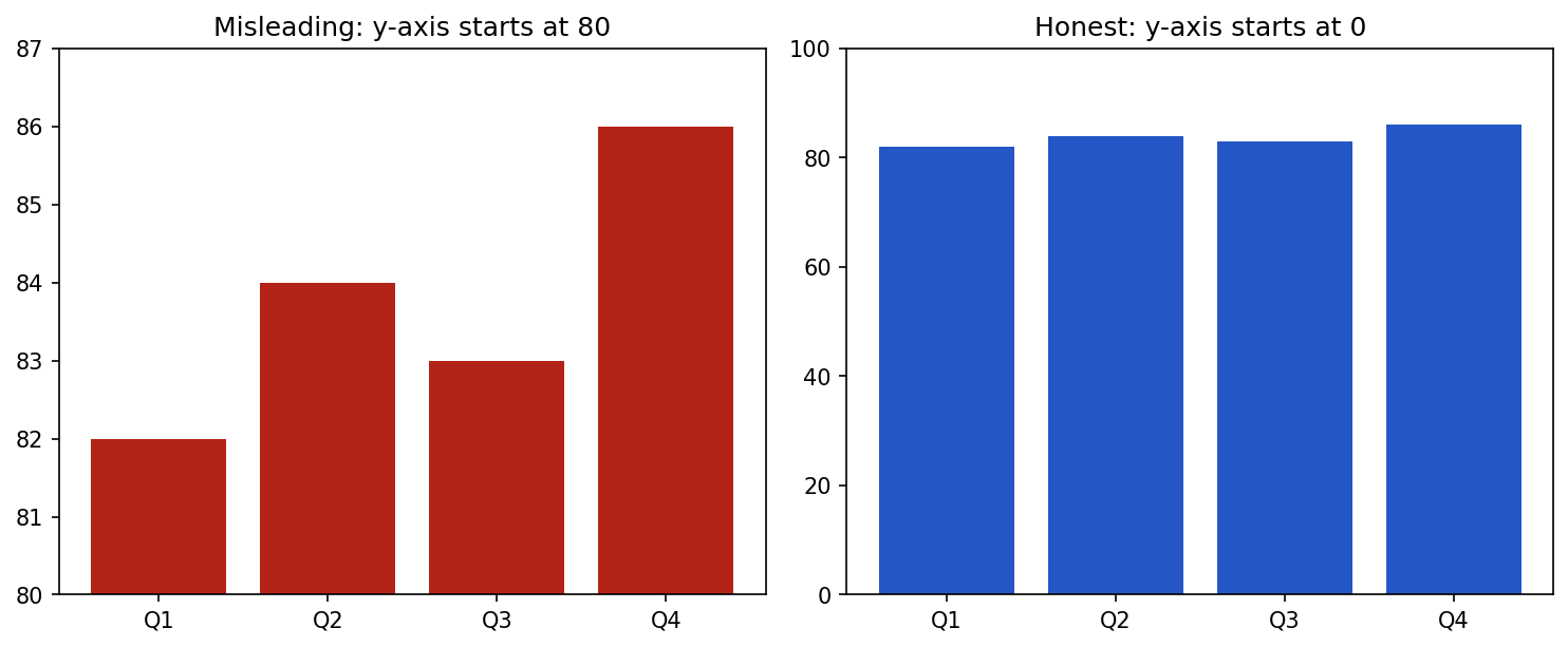
- Be honest. Start bar-chart axes at zero; do not crop to exaggerate a difference.
The same data can mislead or inform depending on these choices. Clutter buries the message:
Show the code that generated this plot
import numpy as np
import matplotlib.pyplot as plt

categories = ['Site A', 'Site B', 'Site C', 'Site D', 'Site E']
values = [12, 19, 9, 25, 15]

fig, (ax1, ax2) = plt.subplots(1, 2, figsize=(11, 4.4))

# Cluttered: rainbow colors, heavy grid, unsorted, no focus
ax1.bar(categories, values, color=['#e6194b', '#3cb44b', '#ffe119', '#4363d8', '#f58231'])
ax1.grid(True, color='#9aa5b1', linewidth=1.2)
ax1.set_title('Cluttered')

# Clean: sorted, highlight the max, minimal chrome
order = np.argsort(values)[::-1]
cats = [categories[i] for i in order]
vals = [values[i] for i in order]
colors = ['#2457c5' if v == max(vals) else '#cbd5e1' for v in vals]
ax2.bar(cats, vals, color=colors)
ax2.set_ylabel('defect rate (%)')
for spine in ('top', 'right'):
    ax2.spines[spine].set_visible(False)
ax2.set_title('Clean')
plt.show()
Two specific principles are easiest to see side by side. First, start the axis at zero — a truncated axis turns a tiny difference into a dramatic one:
Show the code that generated this plot
import matplotlib.pyplot as plt
quarters = ['Q1', 'Q2', 'Q3', 'Q4']
values = [82, 84, 83, 86]
fig, (ax1, ax2) = plt.subplots(1, 2, figsize=(10, 4.2))
ax1.bar(quarters, values, color='#b42318')
ax1.set_ylim(80, 87) # truncated axis exaggerates the difference
ax1.set_title('Misleading: y-axis starts at 80')
ax2.bar(quarters, values, color='#2457c5')
ax2.set_ylim(0, 100) # honest zero baseline
ax2.set_title('Honest: y-axis starts at 0')
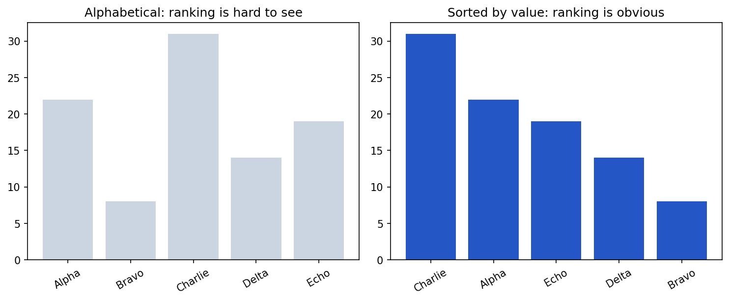
plt.show()Second, order bars by value so the ranking reads instantly:
Show the code that generated this plot
import numpy as np
import matplotlib.pyplot as plt

cats = ['Alpha', 'Bravo', 'Charlie', 'Delta', 'Echo']
values = [22, 8, 31, 14, 19]

fig, (ax1, ax2) = plt.subplots(1, 2, figsize=(10, 4.2))
ax1.bar(cats, values, color='#cbd5e1')
ax1.set_title('Alphabetical: ranking is hard to see')

order = np.argsort(values)[::-1]
ax2.bar([cats[i] for i in order], [values[i] for i in order], color='#2457c5')
ax2.set_title('Sorted by value: ranking is obvious')
plt.show()
Exploration versus reporting
These are two different modes, and they call for different charts:
- Exploration is for you. Quick
matplotlibandseabornplots (covered in the Dataset Statistics chapter) to find patterns. Rough is fine. - Reporting is for someone else. Fewer charts, each polished, each with one clear message and full labels. Cut everything that is not part of the point.
A common mistake is to hand a stakeholder an exploration plot — dense, unlabeled, ten series at once — and expect them to find the insight you already know. Do that work for them.
Tell a story, not a data dump
A good report leads with the takeaway, supports it with one or two clean visuals, and states what should happen next. The result of a defect-detection model only changes a decision when the person making it can see, in seconds, what the data says.
Practice Questions
Practice Questions
- What four "jobs" do most charts do, and which chart suits each?
- Why should every chart have a single, stated takeaway?
- Give three ways to remove clutter from a chart.
- Why should a bar chart's value axis usually start at zero?
- What is the difference between an exploration chart and a reporting chart?