Chapter - Algorithm Families
Supplementary chapter prepared for the BWXT Data Science Workforce Training Pilot. This material is original to the program and is not derived from Automate the Boring Stuff with Python; it is written in a similar tone for continuity with the other chapters.
About this chapter
So far, you have learned how to write Python scripts, summarize datasets, visualize patterns, and prepare features for modeling. Those skills help you ask: What information do I have, and is it ready for a model?
This chapter focuses on the next question: What kind of model should I try?
Machine learning algorithms can be grouped into algorithm families. A family is a group of methods that solve similar problems or learn in similar ways. Some algorithms predict numbers. Some predict categories. Some find groups without being told the right answer. Some learn from feedback over time.
The examples in this chapter use manufacturing, inspection, and welding language, but the ideas apply to many kinds of data.
Start with the prediction target
Before choosing an algorithm, identify the target.
The target is the value you want the model to predict, explain, or discover.
Ask:
- Is the target a number?
- Is the target a category?
- Is there a target at all?
- Is the goal to take actions and learn from rewards?
These questions point you toward the right learning framework and algorithm family.
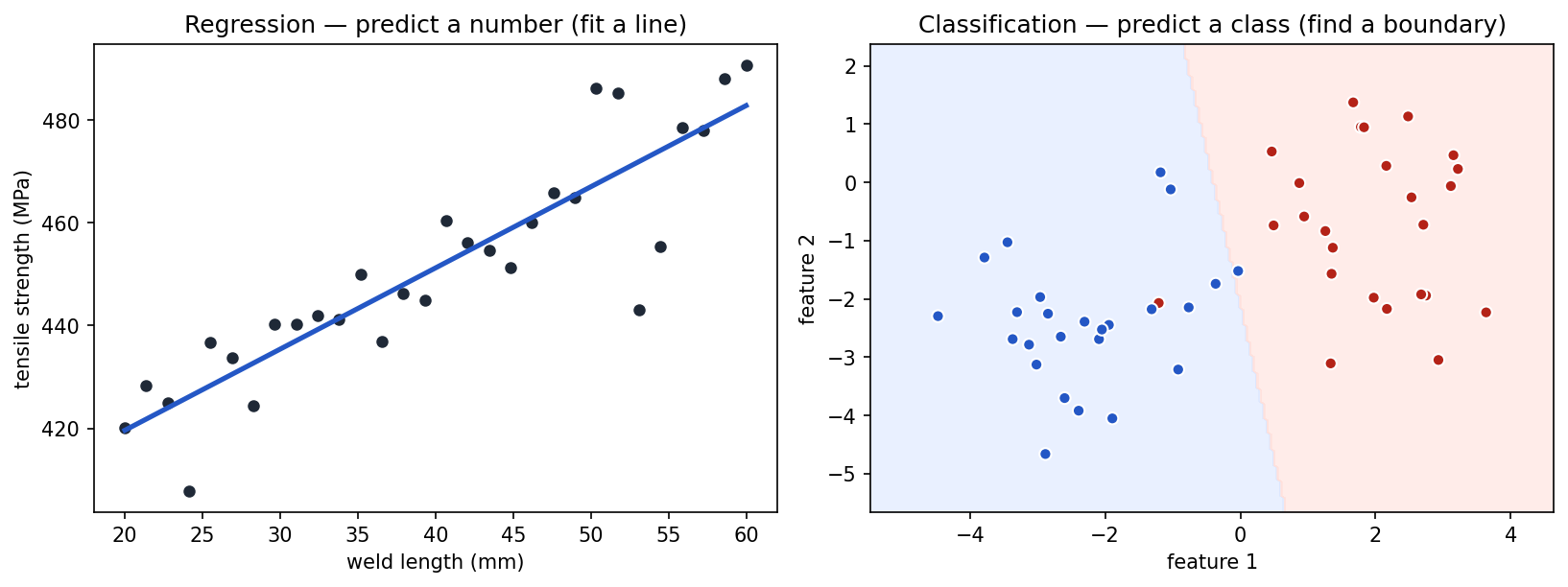
Regression vs. classification
Two of the most common supervised learning problem types are regression and classification.
Show the code that generated this plot
import numpy as np
import matplotlib.pyplot as plt
from sklearn.datasets import make_blobs
from sklearn.linear_model import LogisticRegression

fig, (ax1, ax2) = plt.subplots(1, 2, figsize=(11, 4.2))

# Regression: fit a line through points
rng = np.random.default_rng(1)
x = np.linspace(20, 60, 30)
y = 1.8 * x + 380 + rng.normal(0, 12, size=30)
ax1.scatter(x, y, color='#1f2937', s=25)
ax1.plot(x, np.polyval(np.polyfit(x, y, 1), x), color='#2457c5', linewidth=2.5)
ax1.set_title('Regression — predict a number')

# Classification: learn a boundary between two classes
X, yc = make_blobs(n_samples=50, centers=[[-2, -2], [2, -1]], cluster_std=1.1, random_state=3)
clf = LogisticRegression().fit(X, yc)
xx, yy = np.meshgrid(np.linspace(X[:, 0].min()-1, X[:, 0].max()+1, 200),
                     np.linspace(X[:, 1].min()-1, X[:, 1].max()+1, 200))
Z = clf.predict(np.c_[xx.ravel(), yy.ravel()]).reshape(xx.shape)
ax2.contourf(xx, yy, Z, alpha=0.6)
ax2.scatter(X[:, 0], X[:, 1], c=yc, edgecolor='white', s=35)
ax2.set_title('Classification — find a boundary')
plt.tight_layout()
plt.show()| Problem type | What the model predicts | Example target |
|---|---|---|
| Regression | A numeric value | Weld strength, defect size, remaining useful life |
| Classification | A category or class | pass / fail, defect type, material group |
The difference is not the input data. The same input features might be used for either problem.
For example, these features:
weld_length_mmvoltagetravel_speedmean_pixelmaterial
could be used to predict a numeric target:
tensile_strength_mpa = 485.2That is a regression problem.
The same features could also be used to predict a category:
inspection_result = 'fail'That is a classification problem.
When to use regression
Use regression when the thing you want to predict is numeric and ordered.
Common regression targets include:
- Temperature.
- Pressure.
- Time until failure.
- Defect length.
- Weld strength.
- Cost.
- Probability-like scores, when treated as continuous values.
For example:
target = 'defect_length_mm'If the model predicts 2.5, 3.0, or 7.8, those values have numeric meaning. A prediction of 7.8 mm is larger than 3.0 mm.
Regression models are usually evaluated with metrics such as:
- Mean absolute error.
- Mean squared error.
- Root mean squared error.
- R-squared.
The exact metric should match the practical question. If being wrong by 2 mm is easy to understand, mean absolute error may be useful.
When to use classification
Use classification when the thing you want to predict is a category.
Common classification targets include:
passorfail.defectiveornot_defective.porosity,crack,undercut, orno_defect.low_risk,medium_risk, orhigh_risk.- Material type.
For example:
target = 'defect_class'If the model predicts crack, that is a class label. It is not larger or smaller than porosity. It is simply a different category.
Classification models are usually evaluated with metrics such as:
- Accuracy.
- Precision.
- Recall.
- F1 score.
- Confusion matrix.
- ROC-AUC, especially for binary classification.
The metric matters. In a rare-defect problem, high accuracy can be misleading if the model simply predicts no_defect for almost everything.
A quick decision checklist
Use this checklist before choosing an algorithm:
- Name the target. Write down exactly what the model should predict.
- Check the target type. Is it numeric, categorical, missing, or reward-based?
- Check when the prediction is needed. Do not use features that appear only after the answer is known.
- Check the cost of mistakes. Is a false negative worse than a false positive?
- Start simple. Use a baseline model before trying a complex model.
- Compare fairly. Train and test models using the same data split and metric.
Learning frameworks
A learning framework describes how the model receives information.
| Framework | What the model learns from | Common goal |
|---|---|---|
| Supervised learning | Examples with known answers | Predict a target |
| Unsupervised learning | Examples without known answers | Find structure |
| Self-supervised learning | Labels created from the data itself | Learn useful representations |
| Reinforcement learning | Actions, rewards, and feedback | Learn a policy for decisions |
These frameworks are not competing answers to every problem. They solve different kinds of problems.
Supervised learning
In supervised learning, the training data includes inputs and known answers.
For example:
| weld_id | voltage | travel_speed | defect_class |
|---|---|---|---|
| W001 | 22.1 | 4.8 | no_defect |
| W002 | 19.5 | 5.5 | porosity |
| W003 | 24.3 | 4.1 | crack |
The features are voltage and travel_speed. The label is defect_class.
Supervised learning is useful when:
- You have reliable labels.
- You know what you want to predict.
- Future examples will look similar to training examples.
- You can measure performance against known answers.
Supervised learning has limitations:
- Labels can be expensive or slow to create.
- Bad labels teach the model bad patterns.
- The model may fail when future data differs from training data.
- A model can learn shortcuts if leakage features are present.
Most regression and classification algorithms are supervised learning methods.
Unsupervised learning
In unsupervised learning, the data does not include known answers.
For example, you may have measurements from many welds but no defect labels:
| weld_id | voltage | travel_speed | mean_pixel |
|---|---|---|---|
| W001 | 22.1 | 4.8 | 82.4 |
| W002 | 19.5 | 5.5 | 61.7 |
| W003 | 24.3 | 4.1 | 91.2 |
An unsupervised method might look for groups, unusual examples, or hidden structure.
Unsupervised learning is useful when:
- Labels are not available.
- You want to explore a dataset.
- You want to find clusters or outliers.
- You want to reduce dimensionality before visualization.
Unsupervised learning has limitations:
- There may be no single correct answer.
- Clusters may not match real-world categories.
- Results can be hard to validate.
- Parameter choices can strongly affect the result.
Unsupervised learning is often used early in a project to understand data before building a supervised model.
Self-supervised learning
In self-supervised learning, the model creates a training task from the data itself.
For example, a model might learn from weld images by trying to:
- Predict a missing part of an image.
- Tell whether two image crops came from the same original image.
- Reconstruct a noisy image.
- Predict the next value in a sensor sequence.
The goal is often to learn a useful internal representation before training on a smaller labeled dataset.
Self-supervised learning is useful when:
- You have lots of unlabeled data.
- Labels are expensive.
- You want to pretrain a model before fine-tuning.
- The raw data has structure, such as images, text, audio, or time series.
Self-supervised learning has limitations:
- It can require large datasets and significant computing power.
- The pretraining task may not match the final task.
- It can be harder to explain than simpler supervised methods.
- It usually requires more machine learning engineering.
Self-supervised learning is common in modern computer vision, language models, and sensor-sequence modeling.
Reinforcement learning
In reinforcement learning, an agent learns by taking actions and receiving rewards or penalties.
The model does not simply predict a label. It learns a policy, which is a strategy for choosing actions.
For example, a reinforcement learning setup might involve:
- An agent controlling a simulated robot.
- Actions that move the robot arm.
- Rewards for completing a task safely and accurately.
- Penalties for collisions, delays, or wasted motion.
Reinforcement learning is useful when:
- The problem involves sequences of decisions.
- Actions affect future states.
- A simulator or safe training environment is available.
- The goal can be expressed as a reward.
Reinforcement learning has limitations:
- It can require many trials.
- It can be unstable and hard to debug.
- Poor reward design can teach unwanted behavior.
- It is often risky to train directly on real equipment.
For many manufacturing analytics problems, supervised or unsupervised learning is the better starting point. Reinforcement learning becomes more relevant when the task is about control, planning, or sequential decision-making.
Algorithm families
An algorithm is a specific method for learning from data. An algorithm family is a group of related methods.
This chapter introduces these common families:
- Linear Regression.
- Decision Trees.
- Random Forest.
- Logistic Regression.
- Support Vector Machines.
- Naive Bayes.
- Neural Networks.
- Gradient Boosting.
- Clustering.
No algorithm is best for every problem. The right choice depends on the target, data size, feature types, noise, interpretability needs, and deployment constraints.
Linear Regression
Linear Regression predicts a numeric value by fitting a straight-line relationship between features and the target.
For one feature, the idea looks like this:
predicted_strength = intercept + slope * weld_length_mmWith several features, the model assigns a weight to each feature:
predicted_strength = intercept
                     + weight_1 * voltage
                     + weight_2 * travel_speed
                     + weight_3 * heat_input
Linear Regression is usually used for regression problems.
Example:
from sklearn.linear_model import LinearRegression

X = df[['voltage', 'travel_speed', 'heat_input']]
y = df['tensile_strength_mpa']

model = LinearRegression()
model.fit(X, y)

predictions = model.predict(X)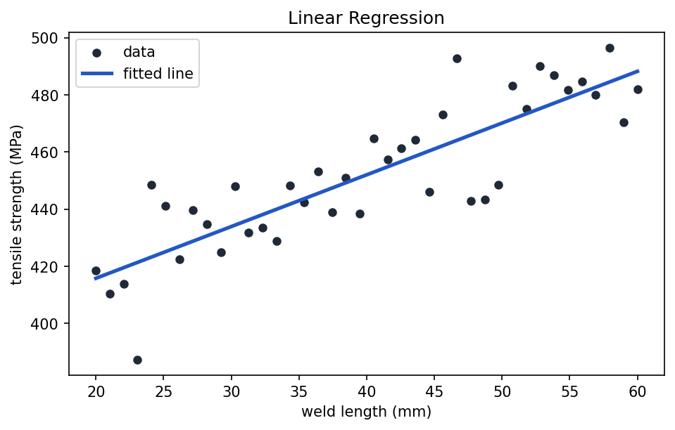
Show the code that generated this plot
import numpy as np
import matplotlib.pyplot as plt
from sklearn.linear_model import LinearRegression

rng = np.random.default_rng(2)
weld_length_mm = np.linspace(20, 60, 40)
tensile = 1.8 * weld_length_mm + 380 + rng.normal(0, 14, size=40)

model = LinearRegression().fit(weld_length_mm.reshape(-1, 1), tensile)
line = model.predict(weld_length_mm.reshape(-1, 1))

plt.scatter(weld_length_mm, tensile, color='#1f2937', s=25, label='data')
plt.plot(weld_length_mm, line, color='#2457c5', linewidth=2.5, label='fitted line')
plt.xlabel('weld length (mm)')
plt.ylabel('tensile strength (MPa)')
plt.legend()
plt.show()
Linear Regression is useful when:
- The target is numeric.
- You need a simple baseline.
- Relationships are roughly linear.
- Interpretability matters.
- The dataset is not extremely large or complex.
Linear Regression has limitations:
- It struggles with nonlinear patterns unless you create useful features.
- Outliers can strongly affect the fitted line.
- It assumes the target changes in a smooth additive way.
- It may underfit complex data such as images.
Linear Regression is often a good first model for numeric prediction because it is simple and easy to explain.
Logistic Regression
Logistic Regression is used for classification, even though its name includes the word regression.
It takes input features, calculates a score, and passes that score through a sigmoid function to produce a value between 0 and 1.
For binary classification:
probability_of_defect = sigmoid(score)Then a threshold is used to choose a class:
if probability_of_defect >= 0.5:
    predict 'defective'
else:
    predict 'not_defective'
Example:
from sklearn.linear_model import LogisticRegression

X = df[['mean_pixel', 'std_pixel', 'defect_area']]
y = df['is_defective']

model = LogisticRegression()
model.fit(X, y)

predicted_classes = model.predict(X)
predicted_probabilities = model.predict_proba(X)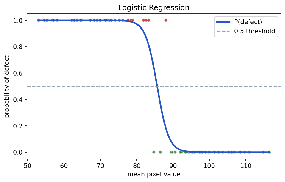
Show the code that generated this plot
import numpy as np
import matplotlib.pyplot as plt
from sklearn.linear_model import LogisticRegression

rng = np.random.default_rng(4)
mean_pixel = np.concatenate([rng.normal(70, 8, 40), rng.normal(100, 8, 40)])
is_defective = np.concatenate([np.ones(40), np.zeros(40)])  # darker -> defect

model = LogisticRegression().fit(mean_pixel.reshape(-1, 1), is_defective)
grid = np.linspace(mean_pixel.min(), mean_pixel.max(), 300).reshape(-1, 1)
prob = model.predict_proba(grid)[:, 1]

plt.scatter(mean_pixel, is_defective, c=is_defective, edgecolor='white', s=30, alpha=0.8)
plt.plot(grid, prob, color='#2457c5', linewidth=2.5, label='P(defect)')
plt.axhline(0.5, color='#94a3b8', linestyle='--', label='0.5 threshold')
plt.xlabel('mean pixel value')
plt.ylabel('probability of defect')
plt.legend()
plt.show()
Logistic Regression is useful when:
- The target is categorical.
- You need a strong simple baseline.
- You want probability-like outputs.
- Interpretability matters.
- Features are already meaningful and well prepared.
Logistic Regression has limitations:
- It draws mostly linear decision boundaries unless features are transformed.
- It may struggle with complex image, text, or sensor patterns.
- It can be sensitive to feature scaling.
- It can perform poorly if classes are not separable using the available features.
Logistic Regression is a common starting point for binary classification.
Decision Trees
A Decision Tree makes predictions by asking a sequence of yes-or-no questions.
For example:
Is mean_pixel < 70?
    yes -> Is defect_area > 12?
        yes -> predict 'defective'
        no  -> predict 'not_defective'
    no  -> predict 'not_defective'
Decision Trees can be used for classification or regression.
Example:
from sklearn.tree import DecisionTreeClassifier

X = df[['mean_pixel', 'std_pixel', 'defect_area']]
y = df['defect_class']

model = DecisionTreeClassifier(max_depth=3, random_state=42)
model.fit(X, y)

predictions = model.predict(X)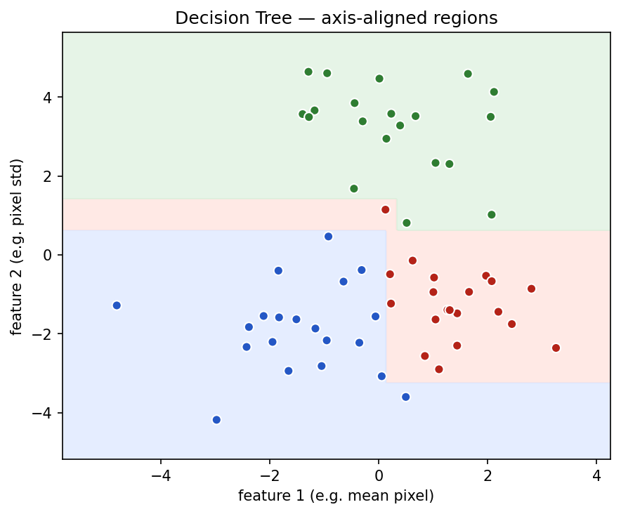
Show the code that generated this plot
import numpy as np
import matplotlib.pyplot as plt
from sklearn.datasets import make_blobs
from sklearn.tree import DecisionTreeClassifier

X, y = make_blobs(n_samples=60, centers=[[-2, -2], [2, -1], [0, 2.5]],
                  cluster_std=1.1, random_state=0)
clf = DecisionTreeClassifier(max_depth=4, random_state=0).fit(X, y)

xx, yy = np.meshgrid(np.linspace(X[:, 0].min()-1, X[:, 0].max()+1, 300),
                     np.linspace(X[:, 1].min()-1, X[:, 1].max()+1, 300))
Z = clf.predict(np.c_[xx.ravel(), yy.ravel()]).reshape(xx.shape)

plt.contourf(xx, yy, Z, alpha=0.7)
plt.scatter(X[:, 0], X[:, 1], c=y, edgecolor='white', s=40)
plt.xlabel('feature 1')
plt.ylabel('feature 2')
plt.title('Decision Tree — axis-aligned regions')
plt.show()
Decision Trees are useful when:
- You want a model that is easy to visualize.
- The data has nonlinear rules.
- Features include mixed scales.
- You want to understand decision paths.
Decision Trees have limitations:
- A deep tree can overfit the training data.
- Small data changes can create a different tree.
- Single trees are often less accurate than ensemble methods.
- Very large trees can become hard to explain.
Decision Trees are helpful teaching models because they match how people often describe rules.
Random Forest
A Random Forest is an ensemble of many Decision Trees.
An ensemble combines multiple models to produce a stronger result. A Random Forest trains many trees on different samples of the data and different subsets of features. The final prediction is based on voting or averaging.
For classification:
tree_1 predicts 'porosity'
tree_2 predicts 'crack'
tree_3 predicts 'porosity'

forest prediction = 'porosity'
Example:
from sklearn.ensemble import RandomForestClassifier

X = df[['mean_pixel', 'std_pixel', 'defect_area']]
y = df['defect_class']

model = RandomForestClassifier(
    n_estimators=100,
    random_state=42,
)
model.fit(X, y)

predictions = model.predict(X)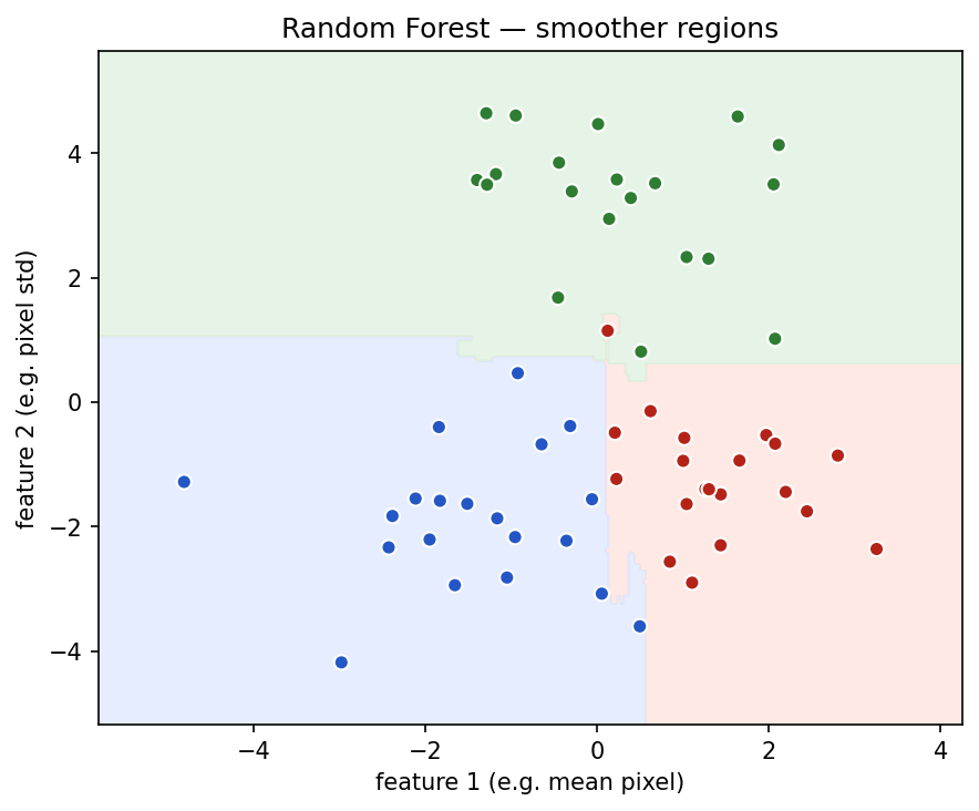
Show the code that generated this plot
import numpy as np
import matplotlib.pyplot as plt
from sklearn.datasets import make_blobs
from sklearn.ensemble import RandomForestClassifier

X, y = make_blobs(n_samples=60, centers=[[-2, -2], [2, -1], [0, 2.5]],
                  cluster_std=1.1, random_state=0)
clf = RandomForestClassifier(n_estimators=200, random_state=0).fit(X, y)

xx, yy = np.meshgrid(np.linspace(X[:, 0].min()-1, X[:, 0].max()+1, 300),
                     np.linspace(X[:, 1].min()-1, X[:, 1].max()+1, 300))
Z = clf.predict(np.c_[xx.ravel(), yy.ravel()]).reshape(xx.shape)

plt.contourf(xx, yy, Z, alpha=0.7)
plt.scatter(X[:, 0], X[:, 1], c=y, edgecolor='white', s=40)
plt.title('Random Forest — smoother regions')
plt.show()
Random Forest is useful when:
- You want strong performance with limited tuning.
- The data has nonlinear patterns.
- You have tabular data with many feature types.
- You want feature importance estimates.
- You want a model less fragile than one Decision Tree.
Random Forest has limitations:
- It is less interpretable than a single tree.
- Large forests can be slower and use more memory.
- Predictions may be less smooth for regression.
- It may not perform as well as gradient boosting on some structured datasets.
Random Forest is a strong general-purpose choice for many tabular classification and regression problems.
Support Vector Machines
Support Vector Machines, or SVMs, try to find a boundary that separates classes with the widest possible margin.
For a binary classification problem, imagine separating two groups of points with a line. The SVM tries to place the line so that it leaves as much space as possible between the classes.
SVMs can also use kernels, which allow them to create nonlinear boundaries.
Example:
from sklearn.pipeline import make_pipeline
from sklearn.preprocessing import StandardScaler
from sklearn.svm import SVC

X = df[['mean_pixel', 'std_pixel', 'defect_area']]
y = df['is_defective']

model = make_pipeline(
    StandardScaler(),
    SVC(kernel='rbf')
)
model.fit(X, y)

predictions = model.predict(X)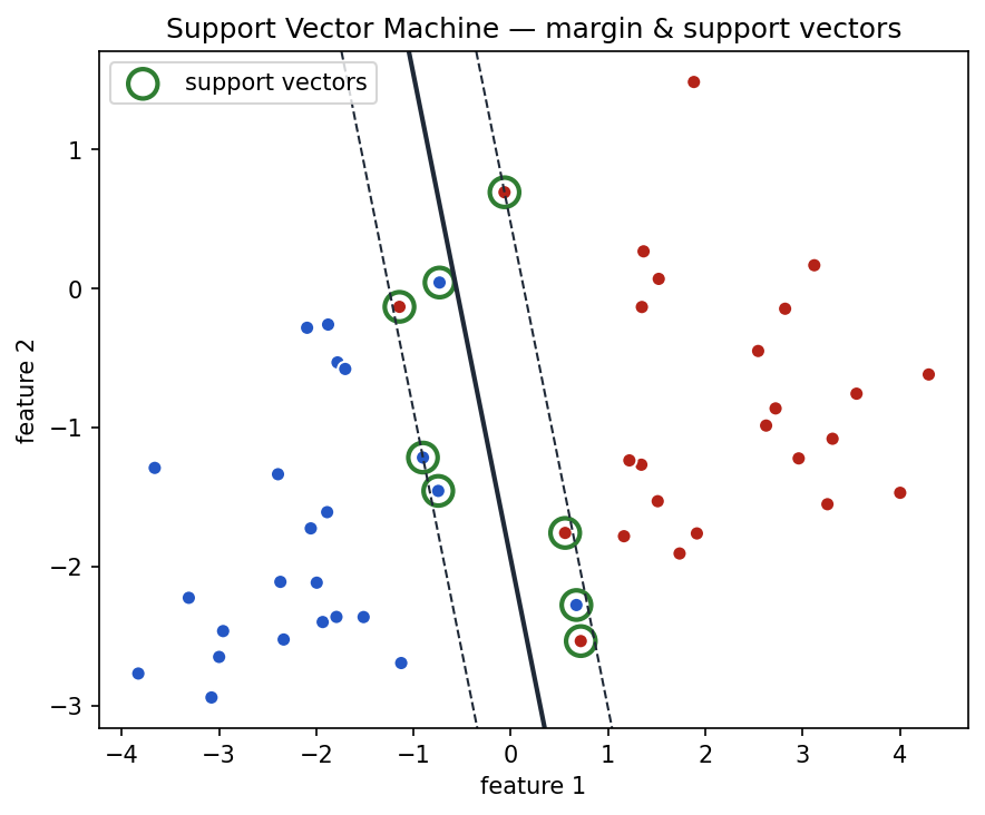
Show the code that generated this plot
import numpy as np
import matplotlib.pyplot as plt
from sklearn.datasets import make_blobs
from sklearn.svm import SVC

X, y = make_blobs(n_samples=50, centers=[[-2, -2], [2, -1]], cluster_std=1.1, random_state=5)
clf = SVC(kernel='linear', C=1.0).fit(X, y)

plt.scatter(X[:, 0], X[:, 1], c=y, edgecolor='white', s=40)
ax = plt.gca()
xx, yy = np.meshgrid(np.linspace(*ax.get_xlim(), 200), np.linspace(*ax.get_ylim(), 200))
Z = clf.decision_function(np.c_[xx.ravel(), yy.ravel()]).reshape(xx.shape)
ax.contour(xx, yy, Z, levels=[-1, 0, 1], colors='#1f2937',
           linestyles=['--', '-', '--'])
ax.scatter(clf.support_vectors_[:, 0], clf.support_vectors_[:, 1],
           s=160, facecolors='none', edgecolors='#2f7d32', linewidths=2)
plt.title('SVM — margin & support vectors')
plt.show()
SVMs are useful when:
- The dataset is small or medium-sized.
- The classes have a clear boundary.
- Feature scaling is handled carefully.
- You want a strong classifier without using a neural network.
- Nonlinear kernels may help separate classes.
SVMs have limitations:
- They can be slow on large datasets.
- They are sensitive to scaling and parameter choices.
- Results can be harder to explain than trees or linear models.
- Probability estimates require extra calibration.
SVMs can work well, but they usually require more care with scaling and tuning than simpler baselines.
Naive Bayes
Naive Bayes is a classification family based on probability.
It estimates how likely each class is given the observed features, then predicts the most likely class.
It is called "naive" because it assumes features are conditionally independent given the class. In real datasets, this assumption is often not perfectly true, but the method can still work surprisingly well.
For example, a text classifier might look at words in an inspection note:
"visible crack near edge"Words such as crack and edge may increase the probability of the crack class.
Example:
from sklearn.naive_bayes import GaussianNB

X = df[['mean_pixel', 'std_pixel', 'defect_area']]
y = df['defect_class']

model = GaussianNB()
model.fit(X, y)

predictions = model.predict(X)
Naive Bayes is useful when:
- You need a fast classification baseline.
- The dataset is small.
- The features are counts, words, or simple measurements.
- You want a model that trains quickly.
- You are working with text classification.
Naive Bayes has limitations:
- The independence assumption may be unrealistic.
- It may underperform when feature interactions matter.
- Probability estimates can be poorly calibrated.
- It is usually not the best choice for complex image patterns.
Naive Bayes is especially useful as a quick baseline and for some text problems.
Neural Networks
Neural Networks are models made of connected layers of simple mathematical units.
Each layer transforms the data into a new representation. With enough data and careful training, neural networks can learn complex patterns in images, text, audio, and sensor sequences.
A simple neural network might take tabular features:
voltage, travel_speed, heat_input -> hidden layers -> defect probabilityA convolutional neural network might take image pixels:
weld image -> image filters -> learned features -> defect classExample:
from sklearn.neural_network import MLPClassifier
from sklearn.pipeline import make_pipeline
from sklearn.preprocessing import StandardScaler

X = df[['mean_pixel', 'std_pixel', 'defect_area']]
y = df['defect_class']

model = make_pipeline(
    StandardScaler(),
    MLPClassifier(hidden_layer_sizes=(32, 16), random_state=42)
)
model.fit(X, y)

predictions = model.predict(X)
Neural Networks are useful when:
- The data has complex nonlinear patterns.
- You have many examples.
- You are working with images, text, audio, or sequences.
- Feature engineering by hand is difficult.
- Predictive performance is more important than simple explanation.
Neural Networks have limitations:
- They often require more data than simpler models.
- They can require significant computing power.
- They can be hard to interpret.
- Training involves many choices, such as architecture and learning rate.
- They can overfit if the dataset is small.
Neural Networks are powerful, but they are not automatically the best choice for every dataset.
Gradient Boosting
Gradient Boosting is an ensemble method that builds models one after another.
Each new model tries to correct mistakes made by the previous models. In many tabular datasets, gradient boosting methods are among the strongest traditional machine learning approaches.
The basic idea:
model_1 makes initial predictions
model_2 learns from model_1's errors
model_3 learns from remaining errors
final prediction combines all models
Example:
from sklearn.ensemble import GradientBoostingClassifier

X = df[['mean_pixel', 'std_pixel', 'defect_area']]
y = df['defect_class']

model = GradientBoostingClassifier(random_state=42)
model.fit(X, y)

predictions = model.predict(X)
Gradient Boosting is useful when:
- You want strong performance on tabular data.
- The data has nonlinear relationships.
- You can spend time tuning parameters.
- You want an ensemble that focuses on hard examples.
- You need classification or regression.
Gradient Boosting has limitations:
- It can overfit if not tuned carefully.
- It can be slower to train than simpler models.
- It has more parameters to understand.
- It is usually less interpretable than a single tree.
Gradient Boosting is often worth trying after simple baselines and Random Forest.
Clustering
Clustering means grouping examples that are similar to each other.
Unlike classification, clustering usually does not use known labels. It is an unsupervised learning method.
For example, clustering might group welds based on sensor measurements:
cluster 0 -> stable process measurements
cluster 1 -> unusually high heat input
cluster 2 -> low brightness images
The cluster numbers do not automatically have real-world meaning. A person still needs to inspect and interpret them.
Example:
from sklearn.cluster import KMeans
from sklearn.pipeline import make_pipeline
from sklearn.preprocessing import StandardScaler

X = df[['voltage', 'travel_speed', 'mean_pixel']]

model = make_pipeline(
    StandardScaler(),
    KMeans(n_clusters=3, random_state=42)
)
cluster_ids = model.fit_predict(X)

df['cluster_id'] = cluster_ids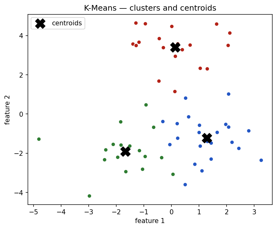
Show the code that generated this plot
import matplotlib.pyplot as plt
from sklearn.datasets import make_blobs
from sklearn.cluster import KMeans

X, _ = make_blobs(n_samples=60, centers=[[-2, -2], [2, -1], [0, 2.5]],
                  cluster_std=1.1, random_state=0)
km = KMeans(n_clusters=3, n_init=10, random_state=0).fit(X)

plt.scatter(X[:, 0], X[:, 1], c=km.labels_, edgecolor='white', s=40)
plt.scatter(km.cluster_centers_[:, 0], km.cluster_centers_[:, 1],
            marker='X', s=220, c='black', label='centroids')
plt.legend()
plt.title('K-Means — clusters and centroids')
plt.show()
Clustering is useful when:
- You do not have labels.
- You want to explore natural groups.
- You want to find unusual examples.
- You want to create rough segments for review.
- You want to compare machine-discovered groups with domain knowledge.
Clustering has limitations:
- The number of clusters may be unclear.
- Different algorithms can produce different groups.
- Scaling can strongly affect results.
- Clusters may not match useful business or engineering categories.
- A cluster label is not the same as a known defect label.
Clustering is best used as an exploration tool unless it has been carefully validated.
Comparing common algorithms
| Algorithm | Common problem type | Strengths | Weaknesses |
|---|---|---|---|
| Linear Regression | Regression | Simple, interpretable, good baseline | Struggles with complex nonlinear patterns |
| Logistic Regression | Classification | Simple, fast, probability-like outputs | Mostly linear boundaries unless features are transformed |
| Decision Trees | Classification or regression | Easy to explain, handles nonlinear rules | Can overfit and be unstable |
| Random Forest | Classification or regression | Strong general-purpose tabular model | Less interpretable and larger than one tree |
| SVMs | Mostly classification | Strong margins, useful on small or medium data | Sensitive to scaling and tuning; slow on large data |
| Naive Bayes | Classification | Very fast, good text baseline | Assumes feature independence |
| Neural Networks | Classification or regression | Learns complex patterns, strong for images and sequences | Needs data, compute, and careful tuning |
| Gradient Boosting | Classification or regression | Often excellent on tabular data | More tuning; can overfit |
| Clustering | Unsupervised grouping | Finds structure without labels | Results can be hard to validate |
This table is a starting point, not a rulebook. Always compare models using the same validation method and the metric that matches the real goal.
Choosing a reasonable first model
For many projects, start with a simple baseline before trying complex methods.
| Situation | Reasonable starting point |
|---|---|
| Numeric target with tabular features | Linear Regression |
| Binary or multi-class label with tabular features | Logistic Regression |
| Nonlinear tabular problem | Decision Tree or Random Forest |
| Strong tabular performance needed | Random Forest or Gradient Boosting |
| Small scaled dataset with clear class boundary | SVM |
| Text classification baseline | Naive Bayes |
| Image classification with enough data | Neural Network |
| No labels and you want groups | Clustering |
Starting simple gives you a baseline. A complex model should earn its place by improving performance, reliability, or usefulness.
Interpreting strengths and weaknesses
When comparing algorithms, do not only ask which one has the highest score.
Also ask:
- Can the model be explained to the people who will use it?
- Does it require features that will be available at prediction time?
- Does it perform well on rare but important cases?
- Is it stable when the data changes slightly?
- How much data does it need?
- How much computing power does it need?
- How difficult will it be to maintain?
For example, a neural network may produce the highest accuracy on weld images, but a Random Forest may be easier to explain for a small tabular dataset. A Logistic Regression model may be less flexible, but it may be enough if the decision boundary is simple.
A practical model-selection workflow
When choosing an algorithm family, use a repeatable workflow.
- Define the target. Decide whether the task is regression, classification, clustering, or something else.
- Inspect the data. Check class counts, missing values, outliers, feature types, and leakage risks.
- Choose a metric. Pick a metric that matches the practical cost of mistakes.
- Build a simple baseline. Use Linear Regression for numeric targets or Logistic Regression for classification when appropriate.
- Try one or two stronger models. For tabular data, Random Forest and Gradient Boosting are common next steps.
- Compare on validation data. Do not judge models only by training performance.
- Inspect errors. Look at examples the model gets wrong.
- Consider explainability and deployment. A slightly less accurate model may be better if it is easier to trust and maintain.
- Document the decision. Record why the selected model was chosen and which alternatives were tested.
Common mistakes
Here are a few traps to avoid:
- Using classification for a numeric target. If the target is
defect_length_mm, regression is usually more natural than turning lengths into arbitrary bins. - Using regression for a category. If the target is
crack,porosity, orno_defect, the model should treat these as classes, not ordered numbers. - Starting with the most complex model. A neural network may not be needed for a small tabular dataset.
- Ignoring class imbalance. A classifier can look accurate while missing rare defects.
- Comparing models using different data splits. Use the same train, validation, and test split for fair comparison.
- Trusting training performance. A model can memorize training data and fail on new examples.
- Assuming clusters are labels. Cluster
0is not automatically a defect type. - Forgetting feature scaling. Algorithms such as SVMs, Logistic Regression, and Neural Networks often need scaled numeric features.
- Choosing only by accuracy. The best model also needs to fit the cost of mistakes, explainability needs, and deployment constraints.
Summary
Algorithm selection begins with the target. If the target is numeric, the problem is usually regression. If the target is a category, the problem is usually classification. If there are no labels and the goal is to find structure, unsupervised learning methods such as clustering may be appropriate.
Supervised learning uses examples with known answers. Unsupervised learning finds structure without known answers. Self-supervised learning creates training tasks from the data itself, often to learn useful representations. Reinforcement learning learns actions from rewards and is most useful for sequential decision-making and control problems.
Common algorithm families include Linear Regression, Logistic Regression, Decision Trees, Random Forest, SVMs, Naive Bayes, Neural Networks, Gradient Boosting, and Clustering. Each has strengths and weaknesses. Good model selection means starting with the problem, building a baseline, comparing fairly, inspecting errors, and documenting the decision.
| Topic | Key ideas |
|---|---|
| Regression | Predicts numeric values |
| Classification | Predicts categories or classes |
| Supervised learning | Learns from labeled examples |
| Unsupervised learning | Finds structure without labels |
| Self-supervised learning | Creates learning signals from the data itself |
| Reinforcement learning | Learns actions from rewards |
| Linear Regression | Simple numeric prediction baseline |
| Logistic Regression | Simple classification baseline |
| Decision Trees | Rule-like model for classification or regression |
| Random Forest | Ensemble of trees; strong tabular model |
| SVMs | Margin-based classifier; sensitive to scaling |
| Naive Bayes | Fast probability-based classifier |
| Neural Networks | Flexible models for complex patterns |
| Gradient Boosting | Sequential ensemble; often strong on tabular data |
| Clustering | Groups similar examples without labels |
Practice Questions
Practice Questions
- In your own words, what is an algorithm family?
- What is the difference between regression and classification?
- If the target is
weld_strength_mpa, is the problem regression or classification? - If the target is
defect_class, is the problem regression or classification? - Why can accuracy be misleading in a rare-defect classification problem?
- What learning framework uses labeled examples?
- What learning framework finds structure without known answers?
- What is one reason self-supervised learning can be useful?
- What kind of problem is reinforcement learning designed for?
- What does Linear Regression predict?
- Why is Logistic Regression used for classification even though it includes the word regression?
- What is one strength and one weakness of a Decision Tree?
- How is a Random Forest different from a single Decision Tree?
- Why do SVMs often require feature scaling?
- What does the "naive" assumption mean in Naive Bayes?
- Name one situation where a Neural Network may be a good choice.
- Name one reason a Neural Network may not be a good first model.
- How does Gradient Boosting build an ensemble?
- What is clustering used for?
- Why should cluster IDs not automatically be treated as real defect labels?
- Choose a reasonable first model for a numeric tabular target and explain why.
- Choose a reasonable first model for a binary classification target and explain why.
- Name two questions you should ask before choosing a model metric.
- Why should models be compared using the same validation split?
- Write a short checklist you would use before selecting an algorithm family for a new welding dataset.