Chapter - Introduction to Neural Networks
Supplementary chapter prepared for the BWXT Data Science Workforce Training Pilot. This material was split out from the CNNs and Computer Vision chapter so learners can study neural-network fundamentals before moving into convolutional models.
About this chapter
This chapter introduces the building blocks shared by many neural-network models, including image models, tabular models, and language models. It covers tensors, neurons, hidden layers, activation functions, losses, weight initialization, backpropagation, and gradient descent.
By the end of this chapter, you should be able to:
- Describe tensors and common tensor shapes.
- Explain perceptrons, neurons, hidden layers, and activation functions.
- Compare ReLU, softplus, threshold, tanh, sigmoid, and softmax.
- Explain why weight initialization affects training stability.
- Choose common loss functions for binary classification, multi-class classification, and regression.
- Describe backpropagation and gradient descent at a high level.
- Adjust a loss choice for practical use cases such as rare critical defects.
Tensors and arrays of different sizes
In deep learning code, images, weights, and activations are usually stored as tensors: multi-dimensional arrays of numbers with a fixed shape (length along each axis).
Think of the rank (number of axes) and the size along each axis:
| Rank | Informal name | Example shape | Example meaning in vision |
|---|---|---|---|
| 0 | Scalar | () |
One number, such as a loss value |
| 1 | Vector | (5,) |
Five scores after a small layer |
| 2 | Matrix | (3, 4) |
A batch of three vectors of length four, or a tiny grayscale patch |
| 3 | 3D array | (3, 32, 32) |
One RGB image: 3 channels, height 32, width 32 (PyTorch-style C×H×W) |
| 4 | 4D array | (16, 3, 224, 224) |
16 images, 3 channels, 224×224 pixels (N×C×H×W, common in PyTorch) |
Channel order depends on the library:
- PyTorch CNNs usually expect NCHW: batch, channels, height, width.
- NumPy plots and many image files are often HWC: height, width, channels.
You must reshape or permute if you convert between conventions.
Small tensors in plain Python (intuition)
A nested list can represent a 2×3 “matrix” (two rows, three columns):
rows = 2
cols = 3
small = [[10 * r + c for c in range(cols)] for r in range(rows)]
# [[0, 1, 2], [10, 11, 12]]
That idea extends to more dimensions, but real models use NumPy or PyTorch so shapes, broadcasting, and hardware acceleration are manageable.
NumPy: shape and common constructors
import numpy as np

a = np.zeros((2, 3))              # 2×3 matrix of zeros
b = np.ones((4,))                  # length-4 vector of ones
c = np.random.randn(3, 3, 3)       # 3×3×3 random values (e.g. a tiny 3-channel volume)
print(a.shape, b.shape, c.shape)
PyTorch: tensors for CNN inputs
In PyTorch, torch.Tensor objects are the usual type for training. Examples of different sizes:
import torch

# Vector of 10 scores (logits for 10 classes)
scores = torch.randn(10)

# One grayscale image: 1 channel, height 28, width 28 (MNIST-style)
gray_one = torch.zeros(1, 28, 28)

# Mini-batch of 32 RGB images, 64×64 (N, C, H, W)
batch = torch.randn(32, 3, 64, 64)

print(scores.shape, gray_one.shape, batch.shape)
Reshaping (same total number of elements)
Changing shape does not change how many numbers you have, only how they are grouped. A length-12 vector can become 3×4 or 2×2×3:
import torch

x = torch.arange(12, dtype=torch.float32)      # 12 elements
y = x.view(3, 4)                                 # 3×4 matrix
z = x.reshape(2, 2, 3)                          # 2×2×3 tensor
# view/reshape require total size to match: 12 = 3*4 = 2*2*3
Use **view** when memory is contiguous; use **reshape** when you want a safe choice that may copy if needed. In image pipelines, reshaping often appears when converting between flattened vectors and feature maps.
For this chapter, the key habit is to always know your tensor shape (especially N, C, H, W) before passing data into a convolution or plotting it.
What is a neural network?
A neural network is a model made of connected layers.
Each layer receives numbers, transforms them, and passes new numbers to the next layer.
A simple network can be described like this:
input features -> hidden layer -> output predictionFor an image model:
image pixels -> feature learning layers -> predictionNeural networks are flexible. They can model complex patterns, but they usually require more data, more computation, and more careful training than simpler models.
Perceptrons and neurons
A perceptron is one of the simplest building blocks of neural networks.
It takes input values, multiplies each by a weight, adds a bias, and produces an output.
For example:
score = weight_1 * input_1
      + weight_2 * input_2
      + weight_3 * input_3
      + bias
In Python-like form:
score = w1 * x1 + w2 * x2 + w3 * x3 + biasThe weights control how much each input matters. The bias shifts the score up or down.
A neuron in a modern neural network usually means this same idea plus an activation function:
neuron output = activation(weighted sum + bias)For example, one neuron might combine image measurements such as:
- Average brightness.
- Pixel contrast.
- Edge strength.
Early neural network layers learn simple patterns. Later layers can combine those patterns into more complex ideas.
Hidden layers
A hidden layer is a layer between the input and output.
It is called hidden because you do not directly provide labels for each hidden layer. The model learns internal representations during training.
For example:
input layer -> hidden layer 1 -> hidden layer 2 -> output layerIn an image model, hidden layers might learn:
| Layer depth | Possible learned pattern |
|---|---|
| Early layers | Edges, corners, simple textures |
| Middle layers | Curves, repeated patterns, local shapes |
| Later layers | Defect-like regions, object parts, high-level visual patterns |
You usually do not hand-code these hidden features. The model learns them from data.
Activation functions
An activation function transforms a neuron's raw score.
Without activation functions, many layers would behave like one large linear model. Activation functions allow neural networks to learn nonlinear patterns.
Common activation functions include:
| Activation | Common use | Basic behavior |
|---|---|---|
| Linear (identity) | Output layer in regression or as a "no activation" pass-through | Returns the input unchanged |
| ReLU | Hidden layers | Keeps positive values, turns negative values into 0 |
| Soft ReLU (softplus) | Hidden layers when a smooth ReLU-like curve is useful | Positive, smooth approximation to ReLU |
| Hard threshold | Rare in end-to-end training | Binary step; not differentiable at the jump |
| Sigmoid | Binary probability-like output | Maps values to 0 through 1 |
| Tanh | Some hidden layers | Maps values to -1 through 1 |
| Softmax | Multi-class output | Converts class scores into class probabilities |
Plotted over a range of inputs, the most common activations look like this:
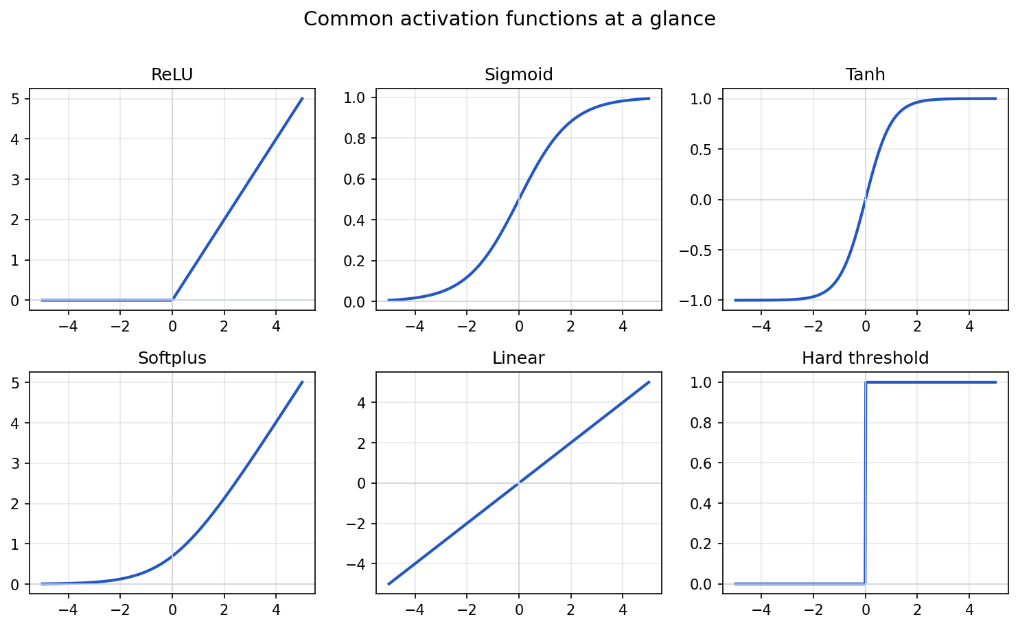
Show the code that generated this plot
import numpy as np
import matplotlib.pyplot as plt

x = np.linspace(-5, 5, 400)
funcs = [
    ('ReLU', np.maximum(0, x)),
    ('Sigmoid', 1 / (1 + np.exp(-x))),
    ('Tanh', np.tanh(x)),
    ('Softplus', np.log1p(np.exp(x))),
    ('Linear', x),
    ('Hard threshold', np.where(x >= 0, 1, 0)),
]

fig, axes = plt.subplots(2, 3, figsize=(10, 6))
for ax, (name, y) in zip(axes.ravel(), funcs):
    ax.plot(x, y, color='#2457c5', linewidth=2)
    ax.set_title(name)
    ax.grid(True, alpha=0.3)
plt.tight_layout()
plt.show()
ReLU
ReLU stands for Rectified Linear Unit.
ReLU(x) = max(0, x)In Python:
def relu(x):
    return max(0, x)


print(relu(-3))
print(relu(5))
Output:
0
5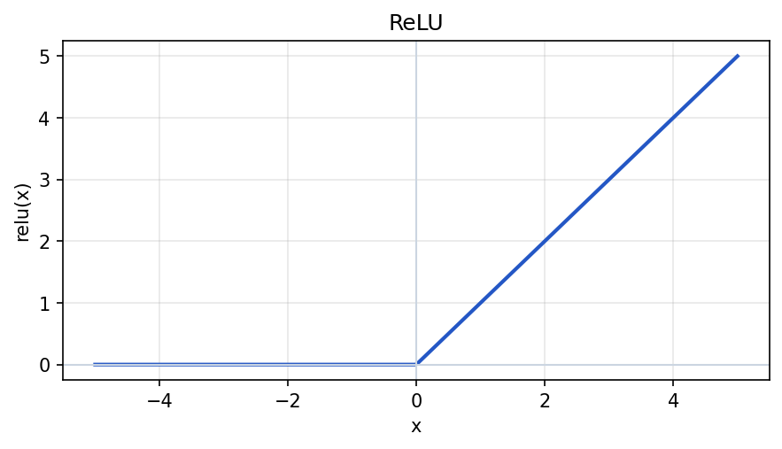
Show the code that generated this plot
import numpy as np
import matplotlib.pyplot as plt

x = np.linspace(-5, 5, 400)
y = np.maximum(0, x)

plt.plot(x, y, color='#2457c5', linewidth=2)
plt.title('ReLU')
plt.xlabel('x')
plt.ylabel('relu(x)')
plt.grid(True, alpha=0.3)
plt.show()
ReLU is common in hidden layers because it is simple and works well in many deep networks.
Linear (identity)
A linear activation is the identity map: the neuron's output is exactly its pre-activation input. It is also called the identity activation.
linear(x) = xIn Python:
def linear(x):
    return x


print(linear(-2.5))
print(linear(7))
Output:
-2.5
7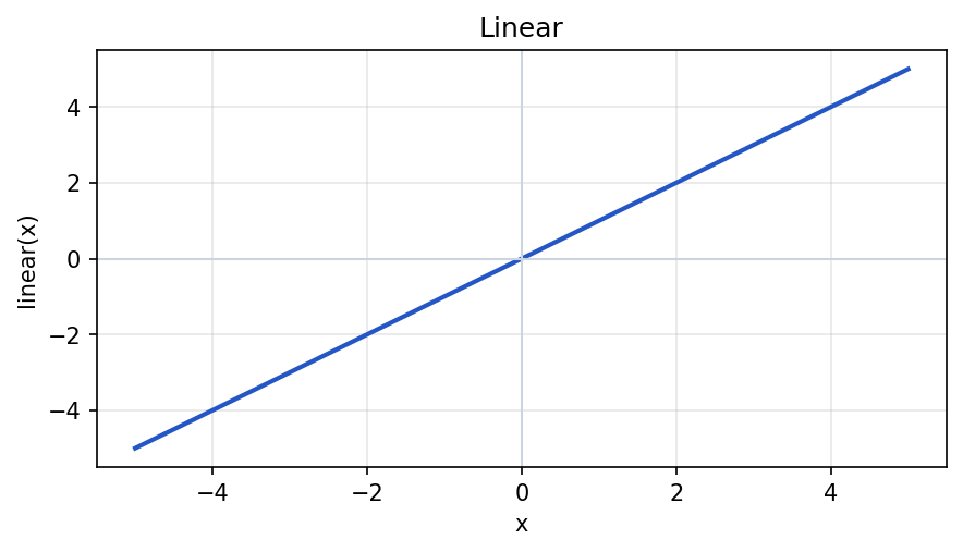
Show the code that generated this plot
import numpy as np
import matplotlib.pyplot as plt

x = np.linspace(-5, 5, 400)
y = x

plt.plot(x, y, color='#2457c5', linewidth=2)
plt.title('Linear')
plt.xlabel('x')
plt.ylabel('linear(x)')
plt.grid(True, alpha=0.3)
plt.show()
Using linear activations everywhere would stack into one large linear transform. In practice, linear is used where you deliberately want no nonlinearity (for example, some output heads in a larger model).
Soft ReLU (softplus)
Soft ReLU often means softplus, a smooth function that behaves like ReLU for large positive inputs but rounds the corner at zero. It is always positive and differentiable everywhere, which can help in some optimization settings.
softplus(x) = ln(1 + exp(x))In Python:
import math


def soft_relu(x):
    """Softplus, a common 'soft' ReLU-style activation."""
    return math.log(1 + math.exp(x))


print(round(soft_relu(-5), 6))
print(round(soft_relu(0), 6))
print(round(soft_relu(3), 6))
Output (rounded):
0.006692
0.693147
3.048587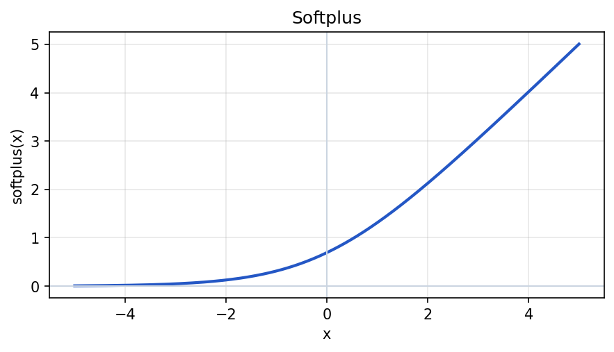
Show the code that generated this plot
import numpy as np
import matplotlib.pyplot as plt

x = np.linspace(-5, 5, 400)
y = np.log1p(np.exp(x))  # log(1 + exp(x)), numerically stable

plt.plot(x, y, color='#2457c5', linewidth=2)
plt.title('Softplus')
plt.xlabel('x')
plt.ylabel('softplus(x)')
plt.grid(True, alpha=0.3)
plt.show()
For large negative x, math.exp(x) underflows and you can use a stable form x + math.log1p(math.exp(-x)) when x is a NumPy or PyTorch tensor. Libraries implement this for you in torch.nn.Softplus and similar.
Hard threshold
A hard threshold (step) maps the score to two values depending on a cutoff. A common convention uses zero:
hard_threshold(x) = 1 if x >= 0 else 0In Python:
def hard_threshold(x):
    return 1 if x >= 0 else 0


print(hard_threshold(-0.1))
print(hard_threshold(0))
print(hard_threshold(2))
Output:
0
1
1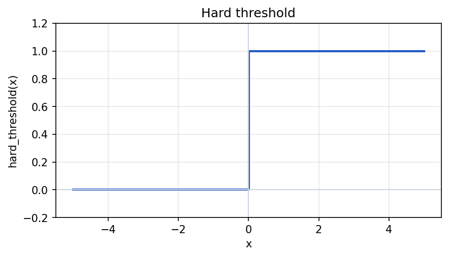
Show the code that generated this plot
import numpy as np
import matplotlib.pyplot as plt

x = np.linspace(-5, 5, 400)
y = np.where(x >= 0, 1, 0)

plt.step(x, y, color='#2457c5', linewidth=2, where='post')
plt.title('Hard threshold')
plt.xlabel('x')
plt.ylabel('hard_threshold(x)')
plt.ylim(-0.2, 1.2)
plt.grid(True, alpha=0.3)
plt.show()
Hard thresholds are not used like ReLU inside standard backpropagation networks because the gradient is zero almost everywhere (and undefined at the jump), so learning does not flow through the input. Perceptron-style training rules are a separate historical case. Some modern networks use softened or stochastic versions instead.
Tanh
The hyperbolic tangent squashes values into the interval -1 through 1, centered at zero. It is sometimes used in hidden layers when zero-centered outputs are desired (unlike sigmoid, which centers near 0.5).
tanh(x) = (exp(x) - exp(-x)) / (exp(x) + exp(-x))In Python (scalar form with math):
import math


def tanh(x):
    return math.tanh(x)


print(tanh(0))
print(round(tanh(1), 6))
print(round(tanh(-2), 6))
Output:
0.0
0.761594
-0.964028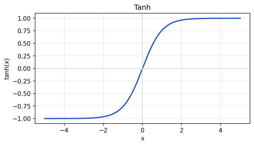
Show the code that generated this plot
import numpy as np
import matplotlib.pyplot as plt

x = np.linspace(-5, 5, 400)
y = np.tanh(x)

plt.plot(x, y, color='#2457c5', linewidth=2)
plt.title('Tanh')
plt.xlabel('x')
plt.ylabel('tanh(x)')
plt.grid(True, alpha=0.3)
plt.show()
Tanh can suffer from vanishing gradients when inputs are very large in magnitude, because the slope of tanh approaches zero in the tails.
Sigmoid
The sigmoid function maps any input to a value between 0 and 1.
It is often used for binary classification outputs.
import math


def sigmoid(x):
    return 1 / (1 + math.exp(-x))


print(sigmoid(0))
print(sigmoid(2))
Output:
0.5
0.8807970779778823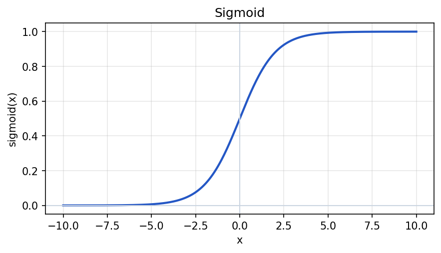
Show the code that generated this plot
import numpy as np
import matplotlib.pyplot as plt

x = np.linspace(-10, 10, 400)
y = 1 / (1 + np.exp(-x))

plt.plot(x, y, color='#2457c5', linewidth=2)
plt.title('Sigmoid')
plt.xlabel('x')
plt.ylabel('sigmoid(x)')
plt.grid(True, alpha=0.3)
plt.show()
If a model outputs 0.88 for "defective," you might interpret that as a high probability-like score.
Softmax
Softmax converts several class scores into values that add up to 1.
It is commonly used for multi-class classification.
For example, a model might output raw scores:
no_defect: 1.2
porosity: 2.5
crack: 0.4
After softmax, the values might look like probabilities:
no_defect: 0.20
porosity: 0.73
crack: 0.07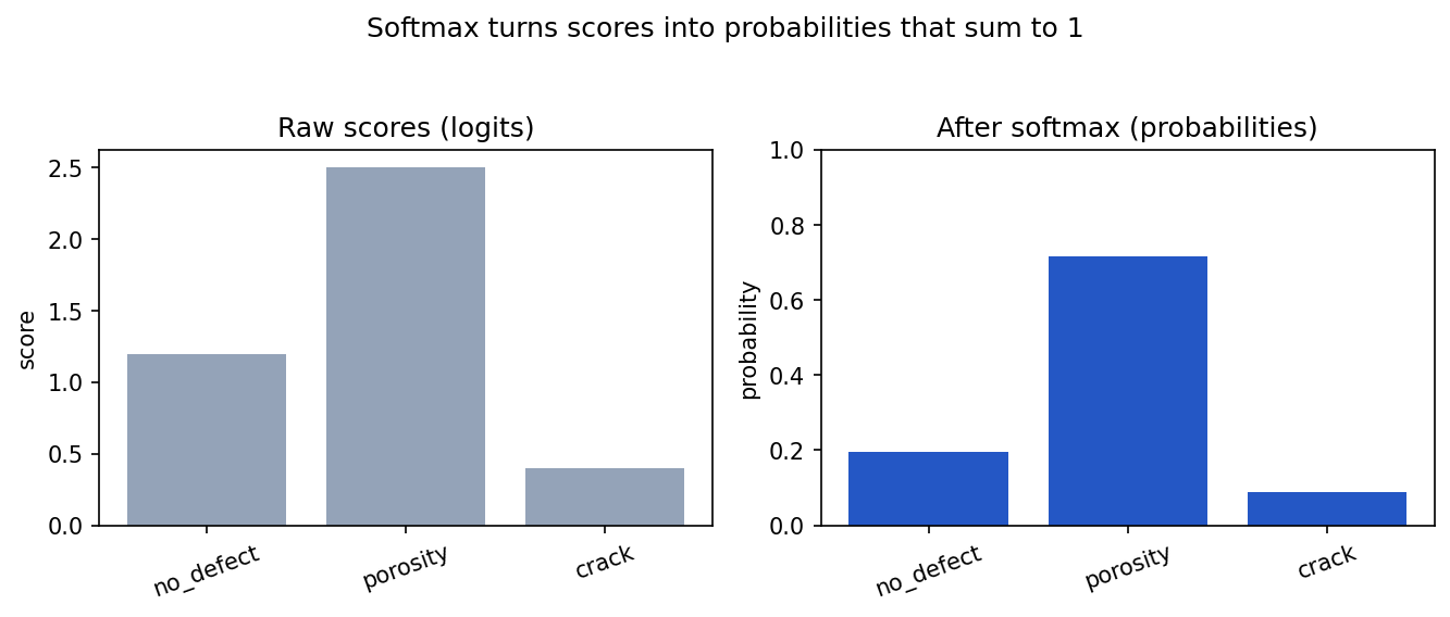
Show the code that generated this plot
import numpy as np
import matplotlib.pyplot as plt

classes = ['no_defect', 'porosity', 'crack']
scores = np.array([1.2, 2.5, 0.4])
probs = np.exp(scores) / np.exp(scores).sum()

fig, (ax1, ax2) = plt.subplots(1, 2, figsize=(9, 3.6))
ax1.bar(classes, scores, color='#94a3b8')
ax1.set_title('Raw scores (logits)')
ax2.bar(classes, probs, color='#2457c5')
ax2.set_title('After softmax (probabilities)')
ax2.set_ylim(0, 1)
plt.tight_layout()
plt.show()
The model would predict porosity because it has the highest value.
Training a neural network
Training means adjusting weights so the model makes better predictions.
A training loop usually follows this pattern:
- Give the model a batch of examples.
- Make predictions.
- Calculate a loss.
- Use backpropagation to calculate how each weight affected the loss.
- Use gradient descent to update the weights.
- Repeat for many batches.
Weight initialization
Before training starts, every weight and bias must have some starting value. That choice is weight initialization. Good initialization helps optimization: the network can learn quickly. Poor initialization can mean flat loss, NaNs, or very slow training.
Why the starting point matters
- All weights zero (or identical): Symmetric layers output the same thing; gradients to each neuron can be identical, so the network may fail to break symmetry and learn diverse features.
- Too large: Activations and gradients can explode layer by layer (numbers grow out of control).
- Too small: Activations and gradients can shrink toward zero in deep networks (vanishing signals), especially with saturating activations.
Deep learning libraries therefore use random initialization, usually drawn from a distribution scaled to the layer width (fan-in / fan-out).
Common schemes (names students see in docs)
| Name | Typical use | Idea in one line |
|---|---|---|
| Uniform / normal, small scale | Older demos, simple nets | Random values with small variance so signals stay moderate at the start. |
| Xavier / Glorot | Layers with tanh or sigmoid | Variance scales like 1 / fan_in (or a fan-in/fan-out average) so linear layers roughly preserve signal scale early in training. |
| He / Kaiming | Layers with ReLU and deep CNNs | Slightly larger variance than Xavier because ReLU zeros out half the activations on average; matches common modern CNN defaults. |
You rarely set these formulas by hand in production. In PyTorch, nn.Linear and nn.Conv2d use Kaiming uniform (He) for ReLU-style defaults unless you change them; other modules may differ. What matters pedagogically is: initialization is not arbitrary—it is tuned so forward passes and gradients stay in a usable numeric range at step zero.
Bias initialization
Biases are often initialized to zero (or a small positive value for ReLU so units can “turn on”). That is usually less critical than weight scaling.
Transfer learning
When you load pretrained weights, you are not using random initialization for those layers—the file supplies the starting point. Only new heads or unfrozen layers rely on fresh initialization or fine-tuning defaults.
Tiny Python illustration (concept only)
import math

fan_in = 256
fan_out = 128
# Xavier / Glorot-style scale (variance ~ 2 / (fan_in + fan_out) for normal in many APIs)
std_xavier = math.sqrt(2.0 / (fan_in + fan_out))
# He / Kaiming-style scale for ReLU (variance ~ 2 / fan_in for normal in PyTorch kaiming_uniform_)
std_he = math.sqrt(2.0 / fan_in)
In practice, call your framework’s built-in initializer (for example reset_parameters on a layer, or nn.init.kaiming_normal_ / xavier_uniform_ in PyTorch) rather than pasting formulas by hand.
Loss functions
A loss function measures how wrong the model is.
The model tries to make the loss smaller during training.
Different tasks need different loss functions.
| Task | Common loss function |
|---|---|
| Binary classification | Binary cross entropy |
| Multi-class classification | Categorical cross entropy or sparse categorical cross entropy |
| Regression | Mean squared error or mean absolute error |
| Object detection boxes | Smooth L1, GIoU, DIoU, or CIoU loss |
| Segmentation masks | Cross entropy, Dice loss, focal loss, or combinations |
Loss is not the same as the final business metric. A model may train with cross entropy but be judged by recall, precision, F1 score, or missed-defect rate.
Binary cross entropy
Binary cross entropy is common when the target has two classes.
Example:
target: defective or not_defectiveIf the true label is defective, the model should output a high probability for defective.
Binary cross entropy penalizes confident wrong predictions more than uncertain wrong predictions.
Why code often clips predictions with a tiny ε (epsilon)
The usual formula uses the predicted probability p (between 0 and 1) and the true label y (often 0 or 1):
loss = -( y * log(p) + (1 - y) * log(1 - p) )If p is exactly 0 or 1, then log(p) or log(1 - p) involves log(0), which is undefined (treats as negative infinity in the limit). That causes numerical overflow, NaNs, and broken gradients during training.
So implementations clip p into a safe interval before taking logs, for example:
p_clipped = min(max(p, ε), 1 - ε)with a very small positive ε, such as 1e-7 or 1e-12. That keeps p_clipped away from 0 and 1 so the logarithms stay finite. The model still learns: extreme predictions are almost unchanged, but the computation stays stable.
This ε is a numerical stability trick, not a change to the idea of cross entropy.
Categorical cross entropy
Categorical cross entropy is common when the target has more than two classes.
Example:
target: no_defect, porosity, crack, or undercutThe model outputs one score for each class. The loss is smaller when the model gives high probability to the correct class.
Mean squared error
Mean squared error, or MSE, is common for regression.
For example, if a model predicts defect length:
true length = 5.0 mm
predicted length = 7.0 mm
error = 2.0 mm
squared error = 4.0
MSE penalizes large errors strongly because errors are squared.
Backpropagation
Backpropagation is the process neural networks use to calculate how each weight contributed to the loss.
It works backward from the output layer through the hidden layers.
For example:
loss -> output layer -> hidden layer 2 -> hidden layer 1 -> input-side weightsBackpropagation answers a question:
If this weight changed slightly, would the loss go up or down?
That information is called a gradient.
You do not usually write backpropagation by hand. Libraries such as PyTorch, TensorFlow, and Keras calculate gradients automatically.
Gradient descent
Gradient descent updates model weights in the direction that reduces loss.
The basic idea:
new weight = old weight - learning_rate * gradientThe learning rate controls how large each update is.
If the learning rate is too small:
- Training may be very slow.
- The model may take a long time to improve.
If the learning rate is too large:
- Training may become unstable.
- The loss may bounce around or get worse.
Gradient descent and backpropagation work together. Backpropagation calculates gradients. Gradient descent uses those gradients to update weights.
Updating a loss function for a use case
Choosing a loss function is not only a math decision. It should match the use case.
Suppose you train a weld image classifier with four classes:
no_defect, porosity, crack, undercutIf all classes are balanced and mistakes have similar cost, ordinary cross entropy may be a reasonable starting point.
But real inspection datasets are often imbalanced. no_defect may be common, while crack may be rare and important.
In that case, ordinary cross entropy might allow the model to perform well overall while missing rare cracks.
Use case: rare critical defects
Use case:
Missing a crack is much worse than incorrectly flagging a clean weld for review.
Possible loss update:
Use weighted cross entropy with a larger class weight for crack.For example:
class_weights = {
    'no_defect': 1.0,
    'porosity': 2.0,
    'undercut': 2.0,
    'crack': 5.0,
}
The exact weights should be chosen through validation, domain review, and error analysis. Higher weight for crack tells the model that crack mistakes are more costly.
Tradeoff:
- Recall for cracks may improve.
- False alarms may increase.
- Overall accuracy may decrease.
That may be acceptable if safety or quality risk makes missed cracks expensive.
Use case: tiny defects in segmentation
Use case:
The model must outline small defect regions, but most pixels are background.
If almost every pixel is background, ordinary pixel-wise cross entropy may encourage the model to predict background too often.
Possible loss update:
Use Dice loss, focal loss, or a combination of cross entropy and Dice loss.Dice loss focuses on overlap between the predicted mask and the true mask.
Focal loss focuses more attention on hard examples and less on easy examples.
Tradeoff:
- Small defect regions may be detected better.
- Training may be more sensitive to parameters.
- The model may require careful threshold tuning.
Loss function decision table
| Use case | Starting loss | Updated loss choice | Why |
|---|---|---|---|
| Balanced binary classification | Binary cross entropy | Binary cross entropy | Classes and error costs are similar |
| Rare critical defect class | Cross entropy | Weighted cross entropy or focal loss | Penalizes missing important rare defects |
| Multi-class defect classification | Cross entropy | Weighted cross entropy | Helps when class counts or costs differ |
| Bounding box regression | Smooth L1 | GIoU, DIoU, or CIoU | Better matches box overlap and geometry |
| Small segmentation masks | Pixel cross entropy | Dice loss or cross entropy plus Dice | Handles small foreground regions better |
| Noisy labels | Cross entropy | Label smoothing or robust loss | Reduces overconfidence on uncertain labels |
Changing the loss function should be tested. A better loss should improve the metric that matters on validation data, not just make the training curve look different.
Summary
Neural networks transform numeric inputs through layers of weighted sums, biases, and activation functions. Tensors keep those numbers organized. Training adjusts weights to reduce a loss function, using backpropagation to compute gradients and gradient descent (or an optimizer based on it) to update parameters. Good initialization, appropriate activations, and a loss function that matches the task are all important for stable learning.
| Topic | Key ideas |
|---|---|
| Tensors | Multi-dimensional arrays used for inputs, weights, activations, and losses |
| Neuron | Weighted sum plus bias, usually followed by an activation function |
| Hidden layer | Internal transformation learned from data |
| Activation | Nonlinear function such as ReLU, sigmoid, tanh, or softmax |
| Initialization | Starting weights affect gradient flow and stability |
| Loss | Measures how wrong the model is for the task |
| Backpropagation | Computes gradients through the network |
| Gradient descent | Updates weights to reduce loss |
Practice Questions
Practice Questions
- What is a tensor?
- Why do neural-network libraries care about shape?
- What does a perceptron compute?
- Why do neural networks need activation functions?
- When would you use sigmoid vs softmax?
- What problem can occur if all weights start at zero?
- Why is He initialization often paired with ReLU?
- What is the difference between binary cross entropy and categorical cross entropy?
- What is backpropagation used for?
- What does gradient descent update?
- Why might rare critical defects require a different loss strategy than common examples?