Chapter - CNNs and Computer Vision
Supplementary chapter prepared for the BWXT Data Science Workforce Training Pilot. This material is original to the program and is not derived from Automate the Boring Stuff with Python; it is written in a similar tone for continuity with the other chapters.
About this chapter
This chapter now focuses specifically on Convolutional Neural Networks (CNNs) and computer-vision task design. If you need a refresher on perceptrons, activations, loss functions, backpropagation, gradient descent, or weight initialization, start with ../Introduction_Neural_Networks/Chapter_Introduction_to_Neural_Networks.md.
By the end of this chapter, you should be able to:
- Describe why images require special handling compared with spreadsheet rows.
- Read common image tensor shapes, especially N×C×H×W vs H×W×C.
- Explain how convolutional filters and pooling operate on image data.
- Describe the structure of a typical CNN classifier.
- Understand the difference between image classification, object detection, and image segmentation.
- Recognize common architectures for each computer-vision task type.
- Explain tradeoffs among common computer-vision architectures.
- Update a vision loss-function strategy based on a practical use case.
Why images are different
A spreadsheet row may have a small number of columns:
| weld_id | voltage | travel_speed | defect_area |
|---|---|---|---|
| W001 | 22.1 | 4.8 | 0.0 |
An image is different. A grayscale image is a grid of pixel values. A color image usually has three channels: red, green, and blue.
For example, a small grayscale image might have shape:
height = 224
width = 224
channels = 1
That is:
224 * 224 * 1 = 50,176 pixel valuesA color image with three channels has:
224 * 224 * 3 = 150,528 pixel valuesImages have spatial structure. Nearby pixels are related. Edges, textures, corners, and shapes matter. CNNs are designed to learn from that structure.
Tensors and arrays of different sizes
In deep learning code, images, weights, and activations are usually stored as tensors: multi-dimensional arrays of numbers with a fixed shape (length along each axis).
Think of the rank (number of axes) and the size along each axis:
| Rank | Informal name | Example shape | Example meaning in vision |
|---|---|---|---|
| 0 | Scalar | () |
One number, such as a loss value |
| 1 | Vector | (5,) |
Five scores after a small layer |
| 2 | Matrix | (3, 4) |
A batch of three vectors of length four, or a tiny grayscale patch |
| 3 | 3D array | (3, 32, 32) |
One RGB image: 3 channels, height 32, width 32 (PyTorch-style C×H×W) |
| 4 | 4D array | (16, 3, 224, 224) |
16 images, 3 channels, 224×224 pixels (N×C×H×W, common in PyTorch) |
Channel order depends on the library:
- PyTorch CNNs usually expect NCHW: batch, channels, height, width.
- NumPy plots and many image files are often HWC: height, width, channels.
You must reshape or permute if you convert between conventions.
Small tensors in plain Python (intuition)
A nested list can represent a 2×3 “matrix” (two rows, three columns):
rows = 2
cols = 3
small = [[10 * r + c for c in range(cols)] for r in range(rows)]
# [[0, 1, 2], [10, 11, 12]]
That idea extends to more dimensions, but real models use NumPy or PyTorch so shapes, broadcasting, and hardware acceleration are manageable.
NumPy: shape and common constructors
import numpy as np

a = np.zeros((2, 3))              # 2×3 matrix of zeros
b = np.ones((4,))                  # length-4 vector of ones
c = np.random.randn(3, 3, 3)       # 3×3×3 random values (e.g. a tiny 3-channel volume)
print(a.shape, b.shape, c.shape)
PyTorch: tensors for CNN inputs
In PyTorch, torch.Tensor objects are the usual type for training. Examples of different sizes:
import torch

# Vector of 10 scores (logits for 10 classes)
scores = torch.randn(10)

# One grayscale image: 1 channel, height 28, width 28 (MNIST-style)
gray_one = torch.zeros(1, 28, 28)

# Mini-batch of 32 RGB images, 64×64 (N, C, H, W)
batch = torch.randn(32, 3, 64, 64)

print(scores.shape, gray_one.shape, batch.shape)
Reshaping (same total number of elements)
Changing shape does not change how many numbers you have, only how they are grouped. A length-12 vector can become 3×4 or 2×2×3:
import torch

x = torch.arange(12, dtype=torch.float32)      # 12 elements
y = x.view(3, 4)                                 # 3×4 matrix
z = x.reshape(2, 2, 3)                          # 2×2×3 tensor
# view/reshape require total size to match: 12 = 3*4 = 2*2*3
Use **view** when memory is contiguous; use **reshape** when you want a safe choice that may copy if needed. In image pipelines, reshaping often appears when converting between flattened vectors and feature maps.
For this chapter, the key habit is to always know your tensor shape (especially N, C, H, W) before passing data into a convolution or plotting it.
What is a CNN?
A Convolutional Neural Network, or CNN, is a neural network designed for image-like data.
CNNs use convolutional layers to scan small filters across an image.
Instead of treating every pixel as unrelated, a CNN learns local visual patterns such as:
- Edges.
- Corners.
- Bright or dark spots.
- Textures.
- Cracks.
- Porosity-like patterns.
The same filter is reused across the image. This helps the model recognize a pattern no matter where it appears.
Convolutional filters
A filter, sometimes called a kernel, is a small grid of weights.
For example, a 3 x 3 filter looks at one small region of an image at a time:
pixel window:
12 15 18
10 14 20
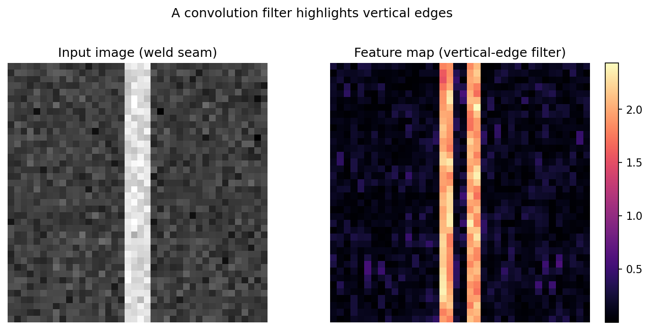
8 11 17The filter slides across the image and produces a new feature map.
Early filters might learn edge detectors. Later filters combine earlier patterns into larger visual structures.
Run on a real image, a vertical-edge filter lights up exactly where brightness changes left-to-right — here, the edges of a weld seam:
Show the code that generated this plot
import numpy as np
import matplotlib.pyplot as plt

# A synthetic grayscale image: a bright vertical weld seam on a noisy plate
rng = np.random.default_rng(0)
image = rng.normal(0.4, 0.05, size=(40, 40))
image[:, 18:22] += 0.5
image = np.clip(image, 0, 1)

# A 3x3 vertical-edge detector (Sobel-style)
kernel = np.array([[-1, 0, 1],
                   [-2, 0, 2],
                   [-1, 0, 1]], dtype=float)

h, w = image.shape
feature_map = np.zeros((h - 2, w - 2))
for i in range(h - 2):
    for j in range(w - 2):
        feature_map[i, j] = np.sum(image[i:i + 3, j:j + 3] * kernel)

fig, (ax1, ax2) = plt.subplots(1, 2, figsize=(9, 4.2))
ax1.imshow(image, cmap='gray');            ax1.set_title('Input image (weld seam)')
ax2.imshow(np.abs(feature_map), cmap='magma'); ax2.set_title('Feature map (vertical-edge filter)')
ax1.axis('off'); ax2.axis('off')
plt.show()
Pooling
Pooling reduces the size of feature maps.
One common type is max pooling, which keeps the largest value in a small region.
For example:
2 x 2 region:
1  4
3  2

max pooled value = 4
Pooling can help by:
- Reducing computation.
- Making the model less sensitive to small shifts.
- Keeping strong visual signals.
Pooling can also discard detail. That matters for tasks such as segmentation, where exact boundaries are important.
A typical CNN classifier
A simple CNN classifier might look like this:
image
-> convolution + ReLU
-> pooling
-> convolution + ReLU
-> pooling
-> dense layer
-> output classFor weld image classification, the output might be:
no_defect, porosity, crack, undercutThe model is not told exactly which pixels form a crack unless the training labels include that information. For ordinary image classification, it only learns from the image-level label.
Updating a loss function for a use case
Choosing a loss function is not only a math decision. It should match the use case.
Suppose you train a weld image classifier with four classes:
no_defect, porosity, crack, undercutIf all classes are balanced and mistakes have similar cost, ordinary cross entropy may be a reasonable starting point.
But real inspection datasets are often imbalanced. no_defect may be common, while crack may be rare and important.
In that case, ordinary cross entropy might allow the model to perform well overall while missing rare cracks.
Use case: rare critical defects
Use case:
Missing a crack is much worse than incorrectly flagging a clean weld for review.
Possible loss update:
Use weighted cross entropy with a larger class weight for crack.For example:
class_weights = {
    'no_defect': 1.0,
    'porosity': 2.0,
    'undercut': 2.0,
    'crack': 5.0,
}
The exact weights should be chosen through validation, domain review, and error analysis. Higher weight for crack tells the model that crack mistakes are more costly.
Tradeoff:
- Recall for cracks may improve.
- False alarms may increase.
- Overall accuracy may decrease.
That may be acceptable if safety or quality risk makes missed cracks expensive.
Use case: tiny defects in segmentation
Use case:
The model must outline small defect regions, but most pixels are background.
If almost every pixel is background, ordinary pixel-wise cross entropy may encourage the model to predict background too often.
Possible loss update:
Use Dice loss, focal loss, or a combination of cross entropy and Dice loss.Dice loss focuses on overlap between the predicted mask and the true mask.
Focal loss focuses more attention on hard examples and less on easy examples.
Tradeoff:
- Small defect regions may be detected better.
- Training may be more sensitive to parameters.
- The model may require careful threshold tuning.
Loss function decision table
| Use case | Starting loss | Updated loss choice | Why |
|---|---|---|---|
| Balanced binary classification | Binary cross entropy | Binary cross entropy | Classes and error costs are similar |
| Rare critical defect class | Cross entropy | Weighted cross entropy or focal loss | Penalizes missing important rare defects |
| Multi-class defect classification | Cross entropy | Weighted cross entropy | Helps when class counts or costs differ |
| Bounding box regression | Smooth L1 | GIoU, DIoU, or CIoU | Better matches box overlap and geometry |
| Small segmentation masks | Pixel cross entropy | Dice loss or cross entropy plus Dice | Handles small foreground regions better |
| Noisy labels | Cross entropy | Label smoothing or robust loss | Reduces overconfidence on uncertain labels |
Changing the loss function should be tested. A better loss should improve the metric that matters on validation data, not just make the training curve look different.
Computer vision task types
Image models can solve different kinds of problems.
Three common task types are:
- Image classification.
- Object detection.
- Image segmentation.
They answer different questions.
| Task | Question answered | Output |
|---|---|---|
| Image classification | What is in this image? | One or more class labels |
| Object detection | What objects are present and where are they? | Boxes plus class labels |
| Image segmentation | Which pixels belong to each class or object? | Pixel-level masks |
Image classification
Image classification assigns a label to an entire image.
Example:
input: weld_001.png
output: porosity
Classification is useful when:
- One label per image is enough.
- You need a simpler annotation process.
- You only need to know whether an image should be routed for review.
Classification has limitations:
- It does not show where the defect is.
- It can struggle if multiple defects appear in one image.
- It may learn shortcuts from backgrounds, lighting, or fixtures.
Common classification architectures
| Architecture | Main idea | Strengths | Weaknesses |
|---|---|---|---|
| LeNet | Early small CNN | Simple, good for teaching | Too small for complex modern images |
| AlexNet | Deeper CNN that helped popularize deep vision models | Historically important, stronger than early CNNs | Large and mostly replaced by newer models |
| VGG | Repeated small convolutions | Simple structure, easy to understand | Many parameters; can be slow and memory-heavy |
| ResNet | Skip connections help train deep networks | Strong baseline, stable deep training | Larger versions can be computationally expensive |
| EfficientNet | Balances depth, width, and resolution | Good accuracy-to-compute tradeoff | More complex design |
| Vision Transformer | Uses attention instead of only convolutions | Strong with large datasets and pretraining | Often needs more data and compute |
For many practical projects, a pretrained ResNet or EfficientNet is a strong starting point.
Object detection
Object detection finds objects and draws boxes around them.
Example:
input: weld_001.png
output:
    class = crack
    box = x, y, width, height
Object detection is useful when:
- You need to know where an object or defect is.
- An image may contain multiple defects.
- A bounding box is detailed enough for the workflow.
Object detection has limitations:
- Box annotations take more time than image labels.
- Boxes are less precise than segmentation masks.
- Small objects can be difficult to detect.
- Models can be more complex to train and evaluate.
Common object detection architectures
Object detectors are often grouped into two-stage and one-stage approaches.
Two-stage detectors
Two-stage detectors first propose possible object regions, then classify and refine them.
Common examples:
- R-CNN.
- Fast R-CNN.
- Faster R-CNN.
- Mask R-CNN, when extended with masks.
Strengths:
- Often accurate.
- Can work well when precise localization matters.
- Good for many object sizes when tuned properly.
Weaknesses:
- Usually slower than one-stage detectors.
- More complex pipeline.
- May be heavier for deployment on limited hardware.
One-stage detectors
One-stage detectors predict boxes and classes in one pass.
Common examples:
- YOLO.
- SSD.
- RetinaNet.
Strengths:
- Often fast.
- Good for real-time or near-real-time workflows.
- Simpler prediction pipeline.
Weaknesses:
- May trade some accuracy for speed.
- Small objects can be challenging.
- Requires careful threshold and anchor or matching choices, depending on the model.
Transformer-based detectors
Transformer-based detectors use attention mechanisms.
Common example:
- DETR.
Strengths:
- Can simplify parts of the detection pipeline.
- Avoids some hand-designed anchor settings.
- Can model global relationships in the image.
Weaknesses:
- May need more data or pretraining.
- Can be slower or harder to tune.
- Training behavior may differ from traditional detectors.
Image segmentation
Image segmentation assigns a class to pixels.
Instead of one label or one box, the model outputs a mask.
Example:
input: weld_001.png
output: pixels belonging to crack
Segmentation is useful when:
- You need exact defect shape or area.
- You need measurements from the detected region.
- Boundaries matter.
- Defects are irregularly shaped.
Segmentation has limitations:
- Pixel-level annotations are time-consuming.
- Small label errors can affect training.
- Models can require more memory.
- Evaluation can be more complex.
Types of segmentation
There are several segmentation task types:
| Type | Meaning | Example |
|---|---|---|
| Semantic segmentation | Assign each pixel a class | All crack pixels are labeled crack |
| Instance segmentation | Separate individual objects | Crack 1 and crack 2 are separate objects |
| Panoptic segmentation | Combines semantic and instance segmentation | Background classes plus separate object instances |
For inspection workflows, semantic segmentation may be enough if you only need defect area. Instance segmentation is useful if you need to count separate defects.
Common segmentation architectures
| Architecture | Main idea | Strengths | Weaknesses |
|---|---|---|---|
| FCN | Fully convolutional network for pixel prediction | Foundational, simpler than many later methods | Coarse outputs without refinement |
| U-Net | Encoder-decoder with skip connections | Strong for medical and industrial images, works with smaller datasets | Can require memory for large images |
| DeepLab | Uses atrous/dilated convolutions for context | Good boundary and context handling | More complex architecture |
| Mask R-CNN | Detection plus instance masks | Good when separate object instances matter | Heavier and needs box/mask annotations |
| SegFormer | Transformer-based segmentation | Strong modern performance | May need more compute and pretraining |
U-Net is a common starting point when you need pixel-level masks for industrial or scientific images.
Choosing the right vision task
Start with the question the user needs answered.
| Need | Task type |
|---|---|
| "Does this image contain a defect?" | Classification |
| "What type of defect is shown?" | Classification |
| "Where is the defect roughly located?" | Object detection |
| "How many defects are present?" | Object detection or instance segmentation |
| "What is the exact defect area?" | Segmentation |
| "Which pixels are crack vs. background?" | Segmentation |
Do not choose segmentation just because it sounds more advanced. If an image-level label is enough, classification may be faster, cheaper, and easier to maintain.
Architecture tradeoffs
When choosing an architecture, consider the full workflow.
| Tradeoff | Classification | Detection | Segmentation |
|---|---|---|---|
| Annotation cost | Lowest | Medium | Highest |
| Output detail | Lowest | Medium | Highest |
| Training complexity | Often lowest | Medium to high | High |
| Inference speed | Often fastest | Depends on detector | Often slower |
| Good for locating defects | No | Yes, with boxes | Yes, with masks |
| Good for measuring exact area | No | Approximate | Yes |
The best architecture is the simplest one that answers the real question well enough.
Common mistakes
Here are a few traps to avoid:
- Using classification when location matters. A class label does not tell you where the defect is.
- Using segmentation when a label is enough. Pixel masks are expensive to label and maintain.
- Ignoring class imbalance. Rare defects may need weighted loss, focal loss, more data, or threshold tuning.
- Choosing a loss function without considering the use case. The loss should support the metric and mistake costs that matter.
- Trusting training loss alone. A low training loss does not prove the model works on new images.
- Ignoring annotation quality. Bad boxes or masks can limit model performance.
- Comparing architectures unfairly. Use the same train, validation, and test splits when comparing models.
- Overlooking deployment constraints. A highly accurate model may be too slow or too large for the production environment.
A practical CNN workflow
When starting a computer vision project, use a repeatable workflow.
- Define the task. Decide whether the problem is classification, detection, or segmentation.
- Inspect the images. Check resolution, lighting, focus, file types, and artifacts.
- Inspect labels. Check class balance, annotation consistency, and missing labels.
- Choose a starting architecture. Use a simple baseline or a pretrained model.
- Choose the loss function. Match the task and use case.
- Train on a small baseline. Confirm the pipeline works before scaling up.
- Evaluate with the right metric. Use recall, precision, F1, IoU, mAP, Dice, or another appropriate measure.
- Review errors with domain experts. Look at false negatives, false positives, and confusing examples.
- Adjust data, loss, thresholds, or architecture. Make changes based on evidence.
- Document decisions. Record why the model, loss, metric, and architecture were chosen.
Summary
CNNs are neural networks designed for grid-like data such as images. Convolutional filters learn local patterns such as edges, textures, corners, and shapes. Pooling can reduce spatial size while keeping strong signals. CNN-based systems may solve classification, object detection, or segmentation tasks depending on what output the workflow requires.
| Topic | Key ideas |
|---|---|
| Image tensor | Numeric grid with height, width, and often channels |
| NCHW / HWC | PyTorch commonly uses batch-channel-height-width; plotting often uses height-width-channel |
| Convolution | Applies learned filters over local regions |
| Pooling | Reduces spatial size while preserving strong responses |
| Classification | Predicts one or more labels for an image |
| Object detection | Predicts boxes and labels for objects |
| Segmentation | Predicts a label for each pixel or region |
| Architecture tradeoff | Accuracy, speed, memory, annotation cost, interpretability |
Practice Questions
Practice Questions
- Why are images different from spreadsheet rows?
- What does N×C×H×W mean?
- Why do convolutional filters help with images?
- What does pooling do?
- What are the main parts of a typical CNN classifier?
- What is the difference between image classification and object detection?
- What is the difference between semantic and instance segmentation?
- When might U-Net be a good starting architecture?
- Why might tiny-defect segmentation need a loss beyond ordinary cross entropy?
- Choose classification, detection, or segmentation for a weld-inspection use case and explain your choice.