Chapter - AI/ML Model Training
Supplementary chapter prepared for the BWXT Data Science Workforce Training Pilot.
About this chapter
Previous chapters introduced data preparation, feature engineering, algorithm families, neural networks, computer vision, and transformer-based systems. This chapter focuses on what happens when you turn those pieces into a repeatable model training process.
Model training is more than calling .fit() one time. A useful model must be trained on the right data, evaluated fairly, compared against alternatives, tuned carefully, documented clearly, and prepared for deployment or further review.
By the end of this chapter, you should be able to:
- Split a dataset intelligently while considering class balance, dataset size, leakage, and the final use case.
- Complete k-fold cross-validation and explain when it is useful.
- Compare model architectures based on the problem definition, functional requirements, and non-functional requirements.
- Communicate model selection decisions to non-technical stakeholders.
- Create a model training pipeline.
- Track model parameters, metrics, artifacts, and results using tools such as MLflow and TensorBoard.
- Adjust model settings to balance accuracy, training time, cost, and operational complexity.
- Iterate on model training until the process is optimized for the problem statement.
- Complete model ensembles using bagging, boosting, and stacking strategies.
- Define and handle overfitting, underfitting, loss curves, and training vs. testing loss curves.
- Determine appropriate decision thresholds based on the use case.
- Understand available compute resources, when to use them, and how to send jobs to run on them.
- Explain the role orchestration and scheduling tools play in model training.
- Describe how distributed training works across multiple GPUs.
The examples in this chapter use manufacturing, inspection, and quality-control language, but the workflow applies to many supervised machine learning projects.
The model training lifecycle
A model training project usually follows a loop:
- Define the problem.
- Collect and inspect the data.
- Split the data.
- Build a simple baseline.
- Train one or more candidate models.
- Evaluate each model on validation data.
- Tune settings and parameters.
- Track every experiment.
- Select a model using technical and stakeholder requirements.
- Test the final model on held-out data.
- Package the pipeline for repeatable use.
- Monitor results after deployment.
This is a loop, not a straight line. Evaluation often reveals problems with features, labels, class balance, architecture choice, or training settings. Good model development is controlled iteration.
Start with the problem statement
Before splitting data or training models, write down the problem in plain language.
For example:
We want to identify weld images that are likely to contain critical defects
so that inspectors can prioritize review.
That problem statement already gives clues:
- The task is probably classification.
- Missing a critical defect may be worse than flagging a good weld.
- The model may need a decision threshold that favors recall.
- The system may be used by inspectors, so explanations and clear reporting matter.
- The model must be evaluated on realistic examples, not only easy training images.
Now compare that with a different problem:
We want to estimate remaining equipment life from sensor readings
so maintenance work can be scheduled earlier.
This is likely a regression or time-to-event problem. The evaluation metric, data split, architecture, and stakeholder message will differ.
Good model training starts with the question: What decision will this model support?
Functional and non-functional requirements
Functional and non-functional requirements: what the system should perform versus how the system should perform
When comparing models, distinguish between functional requirements and non-functional requirements.
Functional requirements describe what the model must do.
Examples:
- Predict whether a part should pass or fail inspection.
- Estimate defect length in millimeters.
- Rank incoming cases by risk.
- Detect a small set of known defect classes.
- Return a confidence score along with the prediction.
Non-functional requirements describe how the model must behave in the real system.
Examples:
- The model must run in less than one second per image.
- Training must finish overnight.
- The model must work on available hardware.
- The model must be explainable enough for review.
- The model must be small enough to deploy to an edge device.
- The model must be maintainable by the team.
- The model must not require data that is unavailable at prediction time.
A model with the highest validation score is not always the best model. It may be too slow, too expensive, too hard to explain, or too fragile.
Intelligent dataset splitting
The goal of data splitting is to estimate how well the model will perform on new data. A careless split can make a model look better than it really is.
Most supervised projects use three groups:
- Training set: used to fit model parameters.
- Validation set: used to compare models, tune settings, and choose thresholds.
- Test set: used once near the end to estimate final performance.
The test set should be treated like future data. Do not repeatedly tune against it.
Overview of train, validation, and test splits plus stratified, grouped, and time-based split strategies
train_test_split() is one of the most important functions in early machine learning work because it creates the first boundary between examples the model is allowed to learn from and examples used to check whether the model generalizes.
Important train_test_split() arguments include:
test_size: controls how much data is held out.train_size: controls how much data is used for training when you prefer to specify that directly.random_state: makes the split repeatable.shuffle: controls whether rows are shuffled before splitting.stratify: preserves the proportions of an important categorical variable.
For most ordinary tabular classification problems, use shuffle=True and stratify=y. For time-ordered problems, do not randomly shuffle future records into the training set.
Common split ratios
There is no single correct ratio. Common starting points include:
70%training,15%validation,15%test.80%training,10%validation,10%test.60%training,20%validation,20%test for smaller datasets.
The right split depends on dataset size.
If you have millions of examples, a small validation percentage may still contain many examples. If you have only a few hundred examples, a large test set may leave too little data for training. In small-data settings, k-fold cross-validation can make better use of the available data.
Stratified splitting for class balance
For classification, preserve class balance when possible. This is called stratification.
Imagine a dataset with 1,000 inspection records:
950 pass
50 fail
If you split randomly without stratification, the validation or test set might contain very few failures. A model could appear accurate while never learning the rare class well.
With scikit-learn:
from sklearn.model_selection import train_test_split

X_train, X_temp, y_train, y_temp = train_test_split(
    X,
    y,
    test_size=0.30,
    stratify=y,
    random_state=42,
)

X_val, X_test, y_val, y_test = train_test_split(
    X_temp,
    y_temp,
    test_size=0.50,
    stratify=y_temp,
    random_state=42,
)
This creates a 70% / 15% / 15% split while keeping class proportions similar in each group.
Stratifying on another feature
Stratification is most often done on the target label, but sometimes another feature also needs balanced representation across splits.
For example, imagine an inspection dataset with an operator_group column, such as trainee, standard, and experienced. If the training set is mostly experienced operators and the test set is mostly trainees, the evaluation may be misleading. Similar concerns can apply to site, machine_type, material, or shift.
If the target is already balanced enough, you may stratify on one important feature:
X_train, X_test, y_train, y_test = train_test_split(
    X,
    y,
    test_size=0.20,
    stratify=df["operator_group"],
    random_state=42,
)
If both the target and another feature matter, create a combined stratification column:
strata = y.astype(str) + "_" + df["operator_group"].astype(str)

X_train, X_test, y_train, y_test = train_test_split(
    X,
    y,
    test_size=0.20,
    stratify=strata,
    random_state=42,
)
Be careful with combined stratification. Every combined group must have enough examples to split. If one group has only one or two rows, train_test_split() may fail or produce an unstable split. In that case, use fewer stratification groups, collect more data, or use grouped cross-validation with careful reporting.
Grouped splitting
Sometimes rows are not independent.
For example:
- Multiple images may come from the same part.
- Multiple measurements may come from the same machine run.
- Multiple records may belong to the same customer, operator, weld, or batch.
If examples from the same group appear in both training and test data, the model may memorize group-specific patterns. This is a form of data leakage.
Use grouped splitting when related examples must stay together.
from sklearn.model_selection import GroupShuffleSplit

splitter = GroupShuffleSplit(
    n_splits=1,
    test_size=0.20,
    random_state=42,
)

train_idx, test_idx = next(splitter.split(X, y, groups=batch_ids))

X_train = X.iloc[train_idx]
X_test = X.iloc[test_idx]
y_train = y.iloc[train_idx]
y_test = y.iloc[test_idx]
Use grouped splitting when the real future use case involves new groups, new batches, new parts, or new sites.
Resampling strategies
Resampling strategies are often used when classes are imbalanced. This chapter does not replace a full feature-engineering or class-imbalance lesson, but the main options are worth reviewing before training.
Common strategies include:
- Oversampling: copy or synthesize more examples from the minority class in the training data.
- Undersampling: remove some examples from the majority class in the training data.
- Synthetic examples: create new minority-class examples, such as with SMOTE for some tabular datasets.
- Class weights: tell the model to penalize mistakes on the minority class more heavily.
- Threshold tuning: keep the same trained model but change the decision threshold.
Apply resampling only to the training data. Do not rebalance the validation or test sets unless you are intentionally creating a separate stress-test dataset. Validation and test sets should usually reflect the real-world distribution.
Time-based splitting
For time series and production systems, random splitting can be misleading. If the model will predict future outcomes, validation and test data should usually come after training data in time.
Example:
Training:   January through August
Validation: September through October
Test:       November through December
This helps answer the practical question: Can the model trained on past data perform well on future data?
Split before fitting transformations
Fit preprocessing steps only on the training data. Then apply those fitted transformations to validation and test data.
This prevents information from validation or test data leaking into training.
Wrong pattern:
scaler.fit(X_all)
X_all_scaled = scaler.transform(X_all)
split_after_scaling = True
Better pattern:
scaler.fit(X_train)
X_train_scaled = scaler.transform(X_train)
X_val_scaled = scaler.transform(X_val)
X_test_scaled = scaler.transform(X_test)
Pipelines help enforce this pattern.
K-fold cross-validation
K-fold cross-validation splits the training data into k parts, called folds. The model trains k times. Each time, one fold is used for validation and the remaining folds are used for training.
For 5 folds:
Run 1: Train on folds 2, 3, 4, 5. Validate on fold 1.
Run 2: Train on folds 1, 3, 4, 5. Validate on fold 2.
Run 3: Train on folds 1, 2, 4, 5. Validate on fold 3.
Run 4: Train on folds 1, 2, 3, 5. Validate on fold 4.
Run 5: Train on folds 1, 2, 3, 4. Validate on fold 5.
The final cross-validation score is usually the mean and standard deviation across folds.
K-fold cross-validation is useful when:
- The dataset is not large.
- You want a more stable estimate than one validation split.
- You are comparing several model types.
- You want to see whether model performance varies a lot depending on the split.
Use StratifiedKFold for classification problems where class balance matters.
from sklearn.model_selection import StratifiedKFold, cross_validate
from sklearn.pipeline import make_pipeline
from sklearn.preprocessing import StandardScaler
from sklearn.linear_model import LogisticRegression

model = make_pipeline(
    StandardScaler(),
    LogisticRegression(max_iter=1000),
)

cv = StratifiedKFold(
    n_splits=5,
    shuffle=True,
    random_state=42,
)

scores = cross_validate(
    model,
    X,
    y,
    cv=cv,
    scoring=["accuracy", "precision", "recall", "f1"],
    return_train_score=True,
)

print(scores["test_f1"].mean())
print(scores["test_f1"].std())
For regression, use KFold instead of StratifiedKFold.
For grouped data, use GroupKFold.
For time-ordered data, use TimeSeriesSplit.
Cross-validation and the final test set
Cross-validation does not remove the need for a final test set. A common workflow is:
- Hold out a final test set.
- Use cross-validation on the remaining training data to compare models and tune settings.
- Choose the final model.
- Train the final model on the full training plus validation data if appropriate.
- Evaluate once on the final test set.
The final test set should not guide repeated decisions.
Build a baseline first
A baseline is a simple model or rule used as a starting point.
Show the code that generated this plot
import numpy as np
import matplotlib.pyplot as plt

epochs = np.linspace(0, 30, 200)
train_err = 0.9 * np.exp(-epochs / 7) + 0.05
val_err = train_err + 0.012 * (epochs - 12) ** 2 / 10
best = epochs[np.argmin(val_err)]

plt.plot(epochs, train_err, color='#2457c5', linewidth=2, label='training error')
plt.plot(epochs, val_err, color='#b42318', linewidth=2, label='validation error')
plt.axvline(best, color='#2f7d32', linestyle='--')        # early-stopping point
plt.axvspan(best, epochs[-1], color='#b42318', alpha=0.06)  # overfitting region
plt.xlabel('Training time (epochs)')
plt.ylabel('Error')
plt.legend()
plt.show()
Examples:
- Predict the most common class.
- Predict the average target value.
- Use Logistic Regression for a classification problem.
- Use Linear Regression for a regression problem.
- Use a small Random Forest for tabular data.
- Use a small CNN or a pretrained model for images.
Baselines answer an important question:
How good is "good enough to be interesting"?If a complex model barely beats a simple baseline, the added complexity may not be worth it.
Compare model architectures
A model architecture is the structure of the model. For traditional machine learning, this may mean the algorithm family and main settings. For neural networks, it usually means the layer design, number of parameters, input shape, and training strategy.
When comparing architectures, consider:
- The problem type.
- The data type.
- The amount of labeled data.
- The metric that matches the real cost of errors.
- Training time.
- Inference speed.
- Explainability.
- Hardware requirements.
- Maintenance complexity.
- Deployment environment.
Tabular data
For tabular data, start simple.
Good first candidates include:
- Logistic Regression for binary or multi-class classification.
- Linear Regression or Ridge Regression for numeric prediction.
- Decision Trees for interpretable nonlinear rules.
- Random Forests for strong general-purpose performance.
- Gradient Boosting for high performance on many structured datasets.
Neural networks can work on tabular data, but they are not automatically better. Tree-based models often perform very well with less tuning.
Image data
For image classification, consider:
- A small CNN when the task is simple and data is limited.
- Transfer learning with a pretrained CNN when data is limited but images resemble common image domains.
- Larger CNNs or vision transformers when data and compute are sufficient.
- Object detection models when the location of defects matters.
- Segmentation models when pixel-level defect regions are needed.
The model should match the output needed by the real workflow. If inspectors only need an image-level pass/fail flag, a segmentation model may be more complex than necessary. If they need defect boundaries for measurement, classification alone may not be enough.
Text and sequence data
For text, consider:
- Bag-of-words plus Logistic Regression as a fast baseline.
- TF-IDF plus linear models for many classification tasks.
- Transformer embeddings when meaning and context are important.
- Fine-tuned transformer models when task-specific performance matters and enough labeled examples are available.
For sensor sequences, consider:
- Feature summaries over time windows.
- Classical time-series models.
- Recurrent neural networks.
- 1D CNNs.
- Transformer-based sequence models.
Start with the simplest model that can reasonably answer the problem.
Communicate model selection to non-technical stakeholders
Non-technical stakeholders usually do not need every algorithm detail. They need to understand what the model does, why it was selected, what it improves, and what it gives up.
A useful explanation covers:
- The decision the model supports.
- The options that were compared.
- The metric used and why it matters.
- The selected model.
- What the selected model gains.
- What the selected model gives up.
- The main risks and how they will be monitored.
Example:
We compared a simple Logistic Regression model, a Random Forest, and a
Gradient Boosting model for predicting whether an inspection record should be
flagged for review. We selected Gradient Boosting because it found more of the
rare failure cases while keeping false alarms at an acceptable level.

What we gain:
- Better detection of likely failures.
- Stronger performance on nonlinear patterns.
- A useful probability score for prioritizing review.

What we give up:
- The model is harder to explain than Logistic Regression.
- Training takes longer.
- We need to monitor feature drift and retrain when the process changes.
This style connects the model decision to business and engineering tradeoffs.
Avoid saying:
We selected XGBoost because it had the best F1 score.That may be technically true, but it does not explain why the score matters or what the organization is accepting in return.
Create a model training pipeline
A training pipeline combines data preparation, feature transformation, model training, and evaluation into a repeatable process.
A pipeline helps prevent mistakes such as:
- Scaling the full dataset before splitting.
- Forgetting to apply the same preprocessing at prediction time.
- Comparing models with different preprocessing.
- Losing track of which settings produced which result.
In scikit-learn:
from sklearn.compose import ColumnTransformer
from sklearn.ensemble import RandomForestClassifier
from sklearn.impute import SimpleImputer
from sklearn.metrics import classification_report
from sklearn.model_selection import train_test_split
from sklearn.pipeline import Pipeline
from sklearn.preprocessing import OneHotEncoder, StandardScaler

numeric_features = ["voltage", "travel_speed", "temperature"]
categorical_features = ["material", "shift"]

numeric_pipeline = Pipeline(
    steps=[
        ("imputer", SimpleImputer(strategy="median")),
        ("scaler", StandardScaler()),
    ]
)

categorical_pipeline = Pipeline(
    steps=[
        ("imputer", SimpleImputer(strategy="most_frequent")),
        ("encoder", OneHotEncoder(handle_unknown="ignore")),
    ]
)

preprocess = ColumnTransformer(
    transformers=[
        ("num", numeric_pipeline, numeric_features),
        ("cat", categorical_pipeline, categorical_features),
    ]
)

model = Pipeline(
    steps=[
        ("preprocess", preprocess),
        ("classifier", RandomForestClassifier(random_state=42)),
    ]
)

X_train, X_test, y_train, y_test = train_test_split(
    X,
    y,
    test_size=0.20,
    stratify=y,
    random_state=42,
)

model.fit(X_train, y_train)
predictions = model.predict(X_test)

print(classification_report(y_test, predictions))
For deep learning, a pipeline may include:
- Dataset loading.
- Data augmentation.
- Batch creation.
- Model initialization.
- Optimizer selection.
- Training loop.
- Validation loop.
- Checkpoint saving.
- Metric logging.
- Final evaluation.
The exact tools differ, but the idea is the same: make training repeatable.
Track experiments with MLflow
Experiment tracking records what happened during training. Without tracking, it becomes difficult to answer:
- Which model produced this score?
- What features were used?
- What learning rate was used?
- Which dataset version was used?
- Which run produced the saved model?
- Did training improve or get worse after a change?
MLflow is a common tool for tracking machine learning experiments. It can log:
- Parameters, such as
learning_rate,max_depth, orbatch_size. - Metrics, such as
accuracy,f1,loss, orrmse. - Artifacts, such as plots, model files, and confusion matrices.
- Models, including scikit-learn, PyTorch, TensorFlow, and other formats.
Example:
import mlflow
import mlflow.sklearn
from sklearn.ensemble import RandomForestClassifier
from sklearn.metrics import accuracy_score, f1_score

mlflow.set_experiment("weld_defect_classification")

with mlflow.start_run():
    n_estimators = 200
    max_depth = 8

    model = RandomForestClassifier(
        n_estimators=n_estimators,
        max_depth=max_depth,
        random_state=42,
    )

    model.fit(X_train, y_train)
    predictions = model.predict(X_val)

    mlflow.log_param("model_type", "RandomForestClassifier")
    mlflow.log_param("n_estimators", n_estimators)
    mlflow.log_param("max_depth", max_depth)

    mlflow.log_metric("accuracy", accuracy_score(y_val, predictions))
    mlflow.log_metric("f1", f1_score(y_val, predictions))

    mlflow.sklearn.log_model(model, "model")
To open the local MLflow UI from a terminal:
mlflow uiThen open the displayed local address in a browser.
Track training with TensorBoard
TensorBoard is especially common for neural network training. It can show:
- Training and validation loss curves.
- Accuracy curves.
- Learning rate changes.
- Histograms of weights.
- Images, text, and embeddings.
- System performance information for some frameworks.
In PyTorch:
from torch.utils.tensorboard import SummaryWriter

writer = SummaryWriter(log_dir="runs/weld_cnn_experiment_01")

for epoch in range(num_epochs):
    train_loss = train_one_epoch(model, train_loader, optimizer)
    val_loss, val_accuracy = evaluate(model, val_loader)

    writer.add_scalar("Loss/train", train_loss, epoch)
    writer.add_scalar("Loss/validation", val_loss, epoch)
    writer.add_scalar("Accuracy/validation", val_accuracy, epoch)

writer.close()
To start TensorBoard:
tensorboard --logdir runsMLflow and TensorBoard can be used together. TensorBoard is often helpful during neural-network training, while MLflow is often helpful for comparing experiment runs and registering model artifacts.
Adjust model settings and parameters
Model settings are often called hyperparameters. They are choices made before or during training that affect how the model learns.
Examples:
max_depthin a decision tree.n_estimatorsin a random forest.learning_ratein gradient boosting or neural networks.batch_sizein neural networks.dropoutrate in neural networks.- Number of layers in a neural network.
- Number of training epochs.
- Regularization strength.
Hyperparameter tuning searches for settings that improve the chosen metric while respecting practical limits.
Where to start
Start with a small, understandable search space. The first tuning run should answer broad questions, not try every possible value.
For example:
- For a decision tree, start with
max_depth,min_samples_leaf, andclass_weight. - For a Random Forest, start with
n_estimators,max_depth, andmin_samples_leaf. - For Gradient Boosting, start with
learning_rate, number of iterations, tree depth, and early stopping. - For neural networks, start with
learning_rate,batch_size, number of epochs, model size, and regularization.
A good starting workflow is:
- Train a simple baseline.
- Pick one stronger model family.
- Tune two or three important hyperparameters.
- Compare the tuned model against the baseline.
- Inspect errors before expanding the search.
Avoid tuning a large grid before you know whether the model family is promising.
Grid search
Grid search tries every combination in a specified list.
from sklearn.model_selection import GridSearchCV
from sklearn.ensemble import RandomForestClassifier

param_grid = {
    "n_estimators": [100, 200, 400],
    "max_depth": [4, 8, None],
    "min_samples_leaf": [1, 5, 10],
}

search = GridSearchCV(
    estimator=RandomForestClassifier(random_state=42),
    param_grid=param_grid,
    scoring="f1",
    cv=5,
    n_jobs=-1,
)

search.fit(X_train, y_train)

print(search.best_params_)
print(search.best_score_)
Grid search is simple but can become expensive quickly.
Random search
Random search samples combinations instead of trying all combinations. It is often more efficient when many settings are possible.
from scipy.stats import randint
from sklearn.model_selection import RandomizedSearchCV

param_distributions = {
    "n_estimators": randint(100, 800),
    "max_depth": [4, 8, 12, None],
    "min_samples_leaf": randint(1, 20),
}

search = RandomizedSearchCV(
    estimator=RandomForestClassifier(random_state=42),
    param_distributions=param_distributions,
    n_iter=25,
    scoring="f1",
    cv=5,
    random_state=42,
    n_jobs=-1,
)

search.fit(X_train, y_train)
For expensive neural-network training, teams may also use Bayesian optimization, early stopping, or specialized hyperparameter tools.
Balance accuracy and training efficiency
The best model is not always the one with the highest score. Training efficiency matters when:
- Training jobs are expensive.
- The model must be retrained often.
- Experiments must finish within a workday or overnight.
- Compute resources are shared.
- A faster model is easier to deploy or maintain.
Useful questions:
- Does doubling training time produce a meaningful improvement?
- Does a larger model help rare but important cases?
- Can we use early stopping?
- Can we reduce image size without losing important information?
- Can we freeze part of a pretrained neural network?
- Can we tune fewer parameters?
- Can we use a smaller model for initial experiments and a larger model later?
For neural networks, common efficiency settings include:
- Smaller batch size when memory is limited.
- Larger batch size when using GPUs efficiently.
- Mixed precision training to reduce memory use and increase speed.
- Early stopping to stop training when validation performance stops improving.
- Checkpointing to save the best model during training.
- Transfer learning to reduce the amount of training needed.
Example early stopping logic:
best_val_loss = float("inf")
epochs_without_improvement = 0
patience = 5

for epoch in range(num_epochs):
    train_loss = train_one_epoch(model, train_loader, optimizer)
    val_loss = evaluate_loss(model, val_loader)

    if val_loss < best_val_loss:
        best_val_loss = val_loss
        epochs_without_improvement = 0
        save_checkpoint(model, "best_model.pt")
    else:
        epochs_without_improvement += 1

    if epochs_without_improvement >= patience:
        print("Stopping early.")
        break
Learning rate that is just right
The learning rate controls how large each training update is. It strongly affects training speed and stability.
If the learning rate is too small:
- Training may be stable but very slow.
- Loss decreases only a little each epoch.
- The model may look like it is underfitting because it has not learned enough yet.
If the learning rate is too large:
- Loss may jump up and down.
- Training may diverge.
- The model may never settle into a useful solution.
If the learning rate is in a good range:
- Training loss decreases steadily.
- Validation loss improves for a while.
- The model reaches useful performance in a reasonable amount of time.
Example pattern:
Too small:   1.00, 0.99, 0.98, 0.97, 0.96
Just right:  1.00, 0.74, 0.55, 0.45, 0.41
Too large:   1.00, 1.80, 0.90, 2.40, 1.30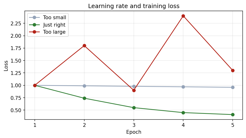
Show the code that generated this plot
import matplotlib.pyplot as plt

epochs = [1, 2, 3, 4, 5]
too_small  = [1.00, 0.99, 0.98, 0.97, 0.96]
just_right = [1.00, 0.74, 0.55, 0.45, 0.41]
too_large  = [1.00, 1.80, 0.90, 2.40, 1.30]

plt.plot(epochs, too_small, marker='o', color='#94a3b8', label='Too small')
plt.plot(epochs, just_right, marker='o', color='#2f7d32', label='Just right')
plt.plot(epochs, too_large, marker='o', color='#b42318', label='Too large')
plt.xlabel('Epoch')
plt.ylabel('Loss')
plt.legend()
plt.show()
Many teams start with a known reasonable value, such as 0.001 for Adam on a neural network, then adjust based on loss curves. Learning-rate schedules can reduce the learning rate during training so the model can make large early progress and smaller later refinements.
Training stability and convergence
A model has converged when additional training produces little or no meaningful improvement. Convergence does not automatically mean the model is good; an underfit model can converge to poor performance.
Training is more stable when:
- Loss generally moves downward instead of jumping wildly.
- Validation metrics improve or level off.
- Repeated runs with the same setup produce similar results.
- Gradients and parameter updates do not explode.
Training may be unstable when:
- Loss becomes
nan. - Loss oscillates sharply.
- Validation metrics change dramatically from epoch to epoch.
- Small changes to the random seed produce very different results.
Useful stability techniques include lowering the learning rate, normalizing inputs, using gradient clipping, increasing batch size when memory allows, checking labels for errors, and simplifying the model.
Iterate until optimized for the problem
Iteration should be structured. Do not change ten things at once unless you are intentionally starting over.
A practical iteration loop:
- Start with a baseline.
- Record baseline metrics.
- Identify the biggest weakness.
- Change one important factor.
- Train again.
- Compare against the baseline.
- Inspect errors.
- Keep the change only if it helps the problem.
- Document the result.
Examples of useful iterations:
- Add class weights for rare failure cases.
- Tune the decision threshold.
- Improve data augmentation for images.
- Remove a leakage feature.
- Add a feature based on domain knowledge.
- Try Random Forest after Logistic Regression.
- Try Gradient Boosting after Random Forest.
- Use transfer learning instead of training a CNN from scratch.
- Reduce model size when inference is too slow.
Every iteration should connect back to the problem statement.
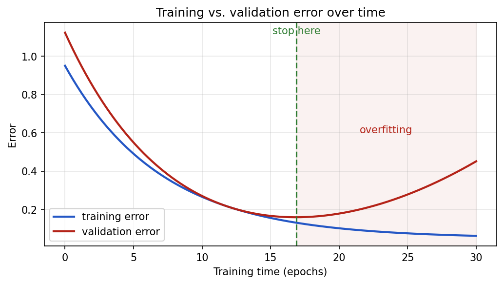
Overfitting
Overfitting happens when a model learns the training data too specifically and does not generalize well to new data.
Signs of overfitting:
- Training loss keeps decreasing while validation loss gets worse.
- Training accuracy is high, but validation accuracy is much lower.
- The model performs well on known examples but poorly on new batches.
- A complex model beats the baseline on training data but not validation data.
Common causes:
- Model is too complex for the amount of data.
- Training for too many epochs.
- Too many weak or noisy features.
- Data leakage.
- Not enough regularization.
- Validation set is too small or not representative.
Ways to reduce overfitting:
- Collect more representative data.
- Use a simpler model.
- Add regularization.
- Use dropout in neural networks.
- Use early stopping.
- Use data augmentation for images.
- Remove leakage features.
- Use cross-validation.
- Prune trees or limit tree depth.
Underfitting
Underfitting happens when a model is too simple or poorly trained to learn the real pattern.
Signs of underfitting:
- Training performance is poor.
- Validation performance is also poor.
- Training and validation losses are both high.
- The model misses obvious patterns.
Common causes:
- Model is too simple.
- Important features are missing.
- Training did not run long enough.
- Learning rate is too low or too high.
- Data preprocessing is incorrect.
- Labels are noisy or inconsistent.
Ways to reduce underfitting:
- Use a more flexible model.
- Add better features.
- Train longer.
- Tune learning rate.
- Reduce excessive regularization.
- Improve label quality.
- Use a pretrained model for complex data such as images or text.
Generalization gap
The generalization gap is the difference between training performance and validation or test performance.
For an error metric such as loss:
generalization_gap = validation_loss - training_lossFor a score where higher is better, such as accuracy or F1:
generalization_gap = training_score - validation_scoreA small gap often means the model is performing similarly on seen and unseen data. A large gap often means the model has learned the training data much better than it handles new examples.
Example:
Training F1:   0.98
Validation F1: 0.71
Gap:           0.27
That gap suggests overfitting or a mismatch between the training and validation data.
Interpret the gap with the absolute scores:
- High training score, low validation score: likely overfitting.
- Low training score, low validation score: likely underfitting or poor data quality.
- High training score, high validation score: likely healthy, but still check the test set.
- Validation score much higher than training score: possible data issue, small validation set, strong regularization, or an easier validation split.
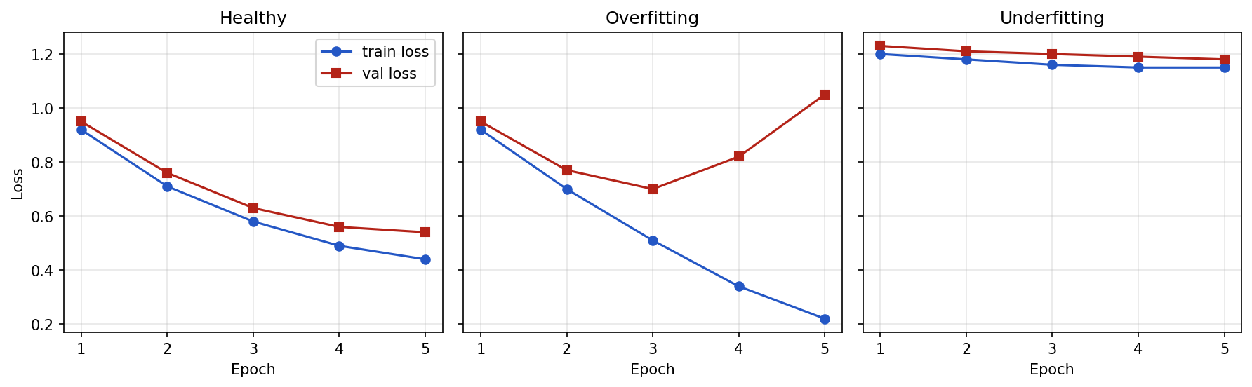
Loss curves
A loss curve shows how the loss changes during training. Loss measures how wrong the model is according to the training objective.
In neural networks, you often plot:
- Training loss by epoch.
- Validation loss by epoch.
- Training accuracy by epoch.
- Validation accuracy by epoch.
Healthy training often looks like this:
Epoch 1:  train_loss = 0.92, val_loss = 0.95
Epoch 2:  train_loss = 0.71, val_loss = 0.76
Epoch 3:  train_loss = 0.58, val_loss = 0.63
Epoch 4:  train_loss = 0.49, val_loss = 0.56
Epoch 5:  train_loss = 0.44, val_loss = 0.54
Both losses decrease, and validation loss stays reasonably close to training loss.
Overfitting may look like this:
Epoch 1:  train_loss = 0.92, val_loss = 0.95
Epoch 2:  train_loss = 0.70, val_loss = 0.77
Epoch 3:  train_loss = 0.51, val_loss = 0.70
Epoch 4:  train_loss = 0.34, val_loss = 0.82
Epoch 5:  train_loss = 0.22, val_loss = 1.05
Training loss improves, but validation loss gets worse.
Underfitting may look like this:
Epoch 1:  train_loss = 1.20, val_loss = 1.23
Epoch 2:  train_loss = 1.18, val_loss = 1.21
Epoch 3:  train_loss = 1.16, val_loss = 1.20
Epoch 4:  train_loss = 1.15, val_loss = 1.19
Epoch 5:  train_loss = 1.15, val_loss = 1.18
Both losses stay high.
Plotted side by side, the three patterns are easy to tell apart:
Show the code that generated this plot
import matplotlib.pyplot as plt

epochs = [1, 2, 3, 4, 5]
healthy   = {'train': [0.92, 0.71, 0.58, 0.49, 0.44], 'val': [0.95, 0.76, 0.63, 0.56, 0.54]}
overfit   = {'train': [0.92, 0.70, 0.51, 0.34, 0.22], 'val': [0.95, 0.77, 0.70, 0.82, 1.05]}
underfit  = {'train': [1.20, 1.18, 1.16, 1.15, 1.15], 'val': [1.23, 1.21, 1.20, 1.19, 1.18]}

fig, axes = plt.subplots(1, 3, figsize=(12, 3.8), sharey=True)
for ax, (title, d) in zip(axes, [('Healthy', healthy), ('Overfitting', overfit), ('Underfitting', underfit)]):
    ax.plot(epochs, d['train'], marker='o', color='#2457c5', label='train loss')
    ax.plot(epochs, d['val'], marker='s', color='#b42318', label='val loss')
    ax.set_title(title)
    ax.set_xlabel('Epoch')
axes[0].set_ylabel('Loss')
axes[0].legend()
plt.tight_layout()
plt.show()
Loss curves help you decide whether to train longer, stop earlier, simplify the model, improve the data, or tune learning settings.
Training vs. testing loss curves
Strictly speaking, you usually track training loss and validation loss during development. The final test set should be used only near the end.
If you repeatedly check test loss during tuning, the test set becomes part of the development process. It is no longer a clean estimate of future performance.
Use this pattern:
- During training: track training loss.
- During model selection: track validation loss and validation metrics.
- After selection: evaluate once on the final test set.
- After deployment: monitor production performance and drift.
If you need long-running monitoring, create a separate monitoring dataset or production feedback process rather than repeatedly tuning on the final test set.
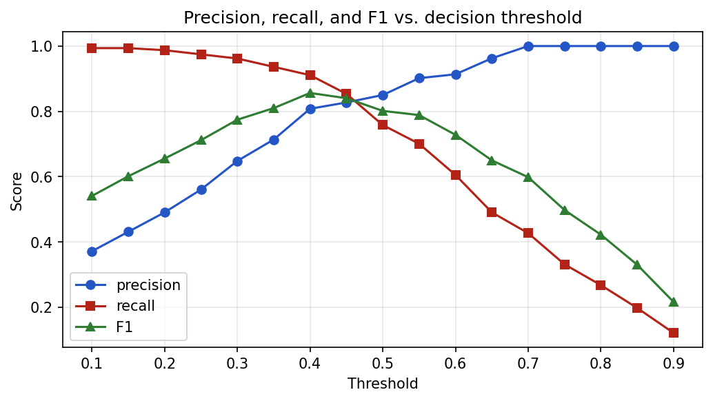
Decision thresholds
Many classifiers produce a probability-like score. A decision threshold converts that score into a class.
For binary classification:
if probability_of_failure >= threshold:
    predict "fail"
else:
    predict "pass"
The default threshold is often 0.5, but it is not always appropriate.
For critical defect detection, you may lower the threshold to catch more possible failures:
threshold = 0.25This may increase recall but also increase false alarms.
For a costly manual review process, you may raise the threshold:
threshold = 0.80This may reduce false alarms but miss more true failures.
Threshold choice should be based on the use case.
Ask:
- What is the cost of a false positive?
- What is the cost of a false negative?
- Does the model support human review or automatic action?
- Is there capacity to review flagged cases?
- Are rare events especially important?
- Does the threshold need to change by product, site, or risk level?
Example threshold search:
import numpy as np
from sklearn.metrics import precision_score, recall_score, f1_score

probabilities = model.predict_proba(X_val)[:, 1]

for threshold in np.arange(0.10, 0.91, 0.05):
    predictions = probabilities >= threshold

    precision = precision_score(y_val, predictions)
    recall = recall_score(y_val, predictions)
    f1 = f1_score(y_val, predictions)

    print(threshold, precision, recall, f1)
Plotting the sweep shows the classic trade-off — raising the threshold lifts precision but lowers recall, and F1 peaks somewhere in between:
Show the code that generated this plot
import numpy as np
import matplotlib.pyplot as plt
from sklearn.metrics import precision_score, recall_score, f1_score

# Synthetic validation set: 1 = failure (rare); the model scores failures higher
rng = np.random.default_rng(7)
y_val = rng.binomial(1, 0.25, size=600)
probabilities = np.clip(0.15 + 0.5 * y_val + rng.normal(0, 0.2, size=600), 0, 1)

thresholds = np.arange(0.10, 0.91, 0.05)
prec, rec, f1 = [], [], []
for t in thresholds:
    pred = probabilities >= t
    prec.append(precision_score(y_val, pred, zero_division=0))
    rec.append(recall_score(y_val, pred, zero_division=0))
    f1.append(f1_score(y_val, pred, zero_division=0))

plt.plot(thresholds, prec, marker='o', color='#2457c5', label='precision')
plt.plot(thresholds, rec, marker='s', color='#b42318', label='recall')
plt.plot(thresholds, f1, marker='^', color='#2f7d32', label='F1')
plt.xlabel('Threshold')
plt.ylabel('Score')
plt.legend()
plt.show()
For stakeholder communication, describe the threshold in plain language:
At this threshold, the model is designed to catch most likely failures, but it
will also send more acceptable parts to manual review. We chose this because
missing a true failure is more costly than reviewing extra parts.
Ensemble models
An ensemble combines multiple models to produce one prediction. Ensembles often improve performance because different models make different errors.
Common ensemble strategies include:
- Bagging.
- Boosting.
- Stacking.
Bagging
Bagging stands for bootstrap aggregating. It trains many models on different samples of the training data and combines their predictions.
Random Forest is a common bagging-based model.
from sklearn.ensemble import RandomForestClassifier

model = RandomForestClassifier(
    n_estimators=300,
    max_depth=None,
    random_state=42,
    n_jobs=-1,
)

model.fit(X_train, y_train)
Bagging is useful when:
- A single model is unstable.
- You want stronger performance than one decision tree.
- You can accept less interpretability than a single tree.
Bagging often reduces variance, which means it can help reduce overfitting compared with one highly flexible model.
Boosting
Boosting trains models sequentially. Each new model focuses more on examples that previous models handled poorly.
Common boosting methods include:
- AdaBoost.
- Gradient Boosting.
- XGBoost.
- LightGBM.
- CatBoost.
In scikit-learn:
from sklearn.ensemble import HistGradientBoostingClassifier

model = HistGradientBoostingClassifier(
    learning_rate=0.05,
    max_iter=300,
    random_state=42,
)

model.fit(X_train, y_train)
Boosting is useful when:
- You need strong tabular performance.
- Nonlinear interactions matter.
- You can tune carefully and monitor overfitting.
Boosting can be very powerful, but it may require more careful tuning than Random Forest.
Stacking
Stacking trains several different base models and then trains a final model to combine their predictions.
Example:
from sklearn.ensemble import RandomForestClassifier, StackingClassifier
from sklearn.linear_model import LogisticRegression
from sklearn.svm import SVC

base_models = [
    ("rf", RandomForestClassifier(n_estimators=200, random_state=42)),
    ("svm", SVC(probability=True, random_state=42)),
]

stacked_model = StackingClassifier(
    estimators=base_models,
    final_estimator=LogisticRegression(max_iter=1000),
    cv=5,
)

stacked_model.fit(X_train, y_train)
Stacking is useful when:
- Different model families perform well in different ways.
- You have enough data for reliable validation.
- You can manage added complexity.
Stacking can improve performance, but it is harder to explain and maintain than a single model.
Compute resources
Model training can run on several types of compute resources.
Common options:
- Local CPU: good for small datasets, simple models, and early experiments.
- Local GPU: useful for neural networks, images, and larger experiments.
- Shared server: useful when the team has a machine with more memory or GPUs.
- Cloud CPU instances: useful for scalable tabular jobs and batch workflows.
- Cloud GPU instances: useful for deep learning, computer vision, and large language model work.
- High-performance computing clusters: useful for large jobs, scheduled workloads, and shared institutional resources.
Choose compute based on:
- Dataset size.
- Model type.
- Training time requirement.
- Memory requirement.
- GPU need.
- Cost.
- Availability.
- Data security requirements.
- Reproducibility needs.
Use a small local run first when possible. It is easier to debug a small job than a large job running on expensive hardware.
When to use a GPU
GPUs are helpful when the training workload involves many parallel numeric operations.
GPUs are usually helpful for:
- CNNs.
- Transformers.
- Large neural networks.
- Large image batches.
- Matrix-heavy deep learning workloads.
GPUs may not help much for:
- Small datasets.
- Simple scikit-learn models.
- Data loading bottlenecks.
- Code that is not written to use GPU libraries.
Before using a GPU, ask:
- Does the model framework support GPU acceleration?
- Is the data pipeline fast enough to keep the GPU busy?
- Does the model fit in GPU memory?
- Is mixed precision appropriate?
- Is the cost justified by the training speed improvement?
In PyTorch:
import torch

device = "cuda" if torch.cuda.is_available() else "cpu"
model = model.to(device)

for features, labels in train_loader:
    features = features.to(device)
    labels = labels.to(device)
    outputs = model(features)
Sending jobs to compute resources
On shared systems, you often submit a training job instead of running it directly in an interactive terminal.
A training script might accept command-line arguments:
import argparse

parser = argparse.ArgumentParser()
parser.add_argument("--learning-rate", type=float, default=0.001)
parser.add_argument("--batch-size", type=int, default=32)
parser.add_argument("--epochs", type=int, default=20)
args = parser.parse_args()

train(
    learning_rate=args.learning_rate,
    batch_size=args.batch_size,
    epochs=args.epochs,
)
Then you can run:
python train.py --learning-rate 0.001 --batch-size 64 --epochs 30On clusters, a scheduler such as SLURM may use a job script:
#!/bin/bash
#SBATCH --job-name=weld-cnn
#SBATCH --gres=gpu:1
#SBATCH --cpus-per-task=8
#SBATCH --mem=32G
#SBATCH --time=04:00:00
#SBATCH --output=logs/%x-%j.out

source .venv/bin/activate
python train.py --batch-size 64 --epochs 30
Then submit:
sbatch train_job.shThe exact commands depend on the compute environment, but the principle is the same: package training into a script that can run repeatably without manual notebook clicks.
Orchestration and scheduling tools
Scheduling decides when and where jobs run. Orchestration coordinates multiple steps in a workflow.
Training workflows often include:
- Data extraction.
- Data validation.
- Feature creation.
- Training.
- Evaluation.
- Model registration.
- Report generation.
- Deployment.
- Monitoring.
Orchestration tools help run these steps in order, retry failures, log outputs, and make workflows repeatable.
Common orchestration and scheduling tools include:
- Cron for simple scheduled scripts.
- SLURM or PBS for cluster jobs.
- Apache Airflow for workflow orchestration.
- Prefect for Python-based workflows.
- Dagster for data and ML workflows.
- Kubeflow for Kubernetes-based ML workflows.
- Cloud-native tools such as AWS Step Functions, Azure Machine Learning pipelines, or Google Vertex AI pipelines.
The infrastructure underneath those tools may include local workstations, shared servers, container images, object storage, model registries, secrets managers, and CPU or GPU clusters. Orchestration connects those pieces so training can run the same way each time instead of depending on manual notebook steps.
Use orchestration when:
- Training has multiple dependent steps.
- Jobs must run on a schedule.
- Jobs need retries and logging.
- Several models must be trained regularly.
- Data refreshes trigger retraining.
- Results must be reproducible and auditable.
Do not start with heavy orchestration for a one-off experiment. Add orchestration when the workflow becomes important enough to repeat reliably.
Distributed training across multiple GPUs
Distributed training uses more than one device or machine to train a model.
The most common strategy is data parallel training:
- Copy the model to each GPU.
- Split each batch across GPUs.
- Each GPU computes gradients on its part of the batch.
- Gradients are synchronized.
- Each model copy is updated consistently.
Distributed training can reduce training time for large models and large datasets, but it adds complexity.
Use distributed training when:
- One GPU is too slow.
- The model or batch size benefits from multiple GPUs.
- The dataset is large enough to keep multiple GPUs busy.
- The team can manage the added debugging and infrastructure.
Avoid distributed training when:
- The model is small.
- Data loading is the bottleneck.
- The dataset is small.
- Single-GPU training already finishes quickly.
- The team has not first validated the training loop on one GPU.
In PyTorch, a common approach is Distributed Data Parallel, usually abbreviated as DDP.
Example launch command:
torchrun --nproc_per_node=4 train.py --epochs 30 --batch-size 128Inside the training code, DDP requires setup such as:
- Initializing the distributed process group.
- Assigning each process to a GPU.
- Wrapping the model with
DistributedDataParallel. - Using a
DistributedSamplerfor the training dataset. - Saving checkpoints from only one process.
Conceptual sketch:
import os
import torch
import torch.distributed as dist
from torch.nn.parallel import DistributedDataParallel

dist.init_process_group(backend="nccl")

local_rank = int(os.environ["LOCAL_RANK"])
torch.cuda.set_device(local_rank)

model = build_model().to(local_rank)
model = DistributedDataParallel(model, device_ids=[local_rank])
Distributed training should be introduced after the single-GPU version is correct and well tracked.
Reproducibility
Reproducibility means someone can understand and, when practical, recreate a training result.
Record:
- Code version.
- Dataset version.
- Train, validation, and test split method.
- Random seed.
- Model architecture.
- Hyperparameters.
- Metric definitions.
- Hardware used.
- Package versions.
- Training time.
- Final model artifact.
Set random seeds when possible:
import random
import numpy as np
import torch

random.seed(42)
np.random.seed(42)
torch.manual_seed(42)
Some GPU operations are not perfectly deterministic by default. Reproducibility is still improved by recording enough information to compare runs fairly.
Common mistakes
Here are a few traps to avoid:
- Splitting after preprocessing. This can leak validation or test information into training.
- Ignoring groups. Examples from the same batch, part, or person can leak across splits.
- Using a random split for future prediction. Time-based problems often need time-based validation.
- Optimizing only accuracy. Accuracy can hide poor rare-class performance.
- Tuning on the test set. This makes the test score overly optimistic.
- Changing many things at once. It becomes difficult to know what helped.
- Not tracking experiments. Results become hard to compare or reproduce.
- Selecting only the highest-scoring model. Deployment, explainability, speed, and cost also matter.
- Using distributed training too early. First make the single-device version correct.
- Forgetting stakeholder tradeoffs. Model selection is both technical and practical.
A practical training checklist
Before training:
- Define the prediction target.
- Define the decision the model supports.
- Choose metrics that match the cost of errors.
- Check class balance.
- Check missing values, outliers, and leakage risks.
- Decide whether the split should be random, stratified, grouped, or time-based.
- Create a final test set.
During training:
- Start with a baseline.
- Use pipelines to keep preprocessing repeatable.
- Track parameters, metrics, artifacts, and code version.
- Compare models on the same validation strategy.
- Watch training and validation loss curves.
- Tune settings in a controlled way.
- Inspect errors, not just scores.
Before final selection:
- Compare functional requirements.
- Compare non-functional requirements.
- Choose a decision threshold based on the use case.
- Explain what is gained and what is given up.
- Evaluate once on the final test set.
- Save the model and preprocessing pipeline together.
- Document the training run.
Concept teaching guide
Use this guide to explain each major concept at several levels. The tiered checks are intentionally short: Tier 1 checks basic recall, Tier 2 checks applied judgment, and Tier 3 checks engineering tradeoffs.
Model training lifecycle
- ELI5: Training a model is like learning to ride a bike: you try, check what went wrong, adjust, and try again until you can ride safely in the real world.
- Teaching one-liner: Model training is an evidence-driven loop, not a one-time
.fit()call. - Tiered comprehension checks:
- Tier 1: Why is training a loop?
- Tier 2: What should you inspect after validation performance is poor?
- Tier 3: How would you decide whether to revisit data, features, architecture, or requirements?
- Failure modes: If you misunderstand the training lifecycle as “load data, train model, report score,” you may trust a model that only looks good because of leakage, a lucky split, bad labels, or the wrong metric. You may also skip baselines, fail to inspect errors, tune blindly, or discover too late that the model does not meet the real engineering requirement.
- Tie to real-world engineering: Production ML teams work in controlled iterations with versioned data, tracked experiments, review gates, and monitoring after deployment.
Functional and non-functional requirements
- ELI5: Functional requirements are the welding defects the model must find; non-functional requirements are how fast, reliable, explainable, and shop-ready the system must be.
- Teaching one-liner: The best model is the one that satisfies both task performance and system constraints.
- Tiered comprehension checks:
- Tier 1: Name one functional and one non-functional requirement.
- Tier 2: Why might the highest-scoring model be rejected?
- Tier 3: How would latency, explainability, hardware, and maintainability affect model selection?
- Failure modes: Focusing only on accuracy can produce a model that is too slow, expensive, fragile, opaque, or impossible to deploy.
- Tie to real-world engineering: Model reviews often compare score, runtime, memory, hardware fit, explainability, retraining burden, and compliance needs together.
Intelligent dataset splitting
- ELI5: Splitting data is like saving some practice questions for the final quiz so you can tell whether you really learned.
- Teaching one-liner: A good split estimates future performance without letting future answers leak into training.
- Tiered comprehension checks:
- Tier 1: What are training, validation, and test sets used for?
- Tier 2: When should you use stratified, grouped, or time-based splitting?
- Tier 3: How would you design a split for rare defects from repeated batches over time?
- Failure modes: Random splits can create leakage, hide rare-class failures, mix related groups, or train on future information.
- Tie to real-world engineering: Reliable ML evaluations depend on splits that match deployment reality, such as new parts, new batches, new sites, or future months.
K-fold cross-validation and final test set
- ELI5: K-fold cross-validation is like letting every student take turns being the quiz checker while still saving one final exam for the end.
- Teaching one-liner: Cross-validation gives a steadier development estimate, but the final test set remains the clean final check.
- Tiered comprehension checks:
- Tier 1: What is a fold?
- Tier 2: Why report mean and standard deviation across folds?
- Tier 3: How would you combine cross-validation with a final held-out test set?
- Failure modes: Using cross-validation scores as the final answer or repeatedly checking the test set can lead to optimistic claims.
- Tie to real-world engineering: Cross-validation helps compare model families on limited data, while a held-out test set supports release decisions and stakeholder reporting.
Baseline model
- ELI5: A baseline is the simple first method you compare against, like asking “How well can our current weld inspection process do before we build something more complex?”
- Teaching one-liner: Build a simple reference point before rewarding complexity.
- Tiered comprehension checks:
- Tier 1: Give one baseline for classification.
- Tier 2: What does it mean if a complex model barely beats the baseline?
- Tier 3: How would a baseline change your recommendation to stakeholders?
- Failure modes: Teams may overbuild, overfit, or spend money on complex models without proving that complexity adds value.
- Tie to real-world engineering: Baselines make model reviews concrete by showing whether added complexity improves outcomes enough to justify cost and maintenance.
Model architecture selection
- ELI5: Choosing an architecture is like choosing the right tool: a hammer, camera, and microscope solve different problems.
- Teaching one-liner: Match the model family to the data type, output needed, constraints, and maintenance burden.
- Tiered comprehension checks:
- Tier 1: Which models are common for tabular data?
- Tier 2: When is segmentation more appropriate than image classification?
- Tier 3: How would you compare a tree model, CNN, and transformer for a constrained deployment?
- Failure modes: Choosing architecture by trend instead of fit can waste compute, reduce explainability, or fail to produce the output users need.
- Tie to real-world engineering: Engineers select architectures by balancing data modality, labeled-data volume, latency, hardware, explainability, deployment target, and retraining plan.
Communicating model selection
- ELI5: Explaining a model is like telling why you picked one route: it is not just fastest, it may be safer or easier to follow.
- Teaching one-liner: Stakeholders need tradeoffs, risks, and decision impact, not only algorithm names or scores.
- Tiered comprehension checks:
- Tier 1: What should a stakeholder explanation include?
- Tier 2: Why is "best F1 score" not enough?
- Tier 3: How would you explain higher recall with more false alarms to an inspection manager?
- Failure modes: Poor communication can cause mistrust, surprise costs, misuse, or rejection of an otherwise useful model.
- Tie to real-world engineering: ML engineers translate metrics into operational consequences such as review workload, missed defects, latency, cost, and monitoring needs.
Model training pipelines
- ELI5: A pipeline is like a recipe card that makes sure every cook follows the same steps in the same order.
- Teaching one-liner: Pipelines make preprocessing, training, and evaluation repeatable and less error-prone.
- Tiered comprehension checks:
- Tier 1: What steps can a pipeline include?
- Tier 2: How do pipelines prevent preprocessing leakage?
- Tier 3: How would you package preprocessing and a model for repeatable retraining and inference?
- Failure modes: Manual notebooks can skip steps, apply different preprocessing at inference, lose settings, or compare models unfairly.
- Tie to real-world engineering: Production ML uses pipelines in scripts, CI jobs, training platforms, and model registries so training and serving transformations stay aligned.
Experiment tracking with MLflow and TensorBoard
- ELI5: Experiment tracking is like keeping a shop notebook for every test weld: you write down the machine settings, material, inspector notes, and results so you know exactly which setup made the best weld.
- Teaching one-liner: Log parameters, metrics, artifacts, and curves so results can be compared and reproduced.
- Tiered comprehension checks:
- Tier 1: What is one parameter and one metric to log?
- Tier 2: When is TensorBoard especially useful?
- Tier 3: How would you use tracked runs to choose and reproduce a final model?
- Failure modes: Without tracking, teams forget which data, code, settings, and artifacts produced a result.
- Tie to real-world engineering: Experiment tracking supports auditability, handoff, model registration, debugging, and rollback when a newer run performs worse.
Hyperparameters, grid search, and random search
- ELI5: Hyperparameters are like oven settings; grid search tries every listed setting, while random search tries a smart sample.
- Teaching one-liner: Tune a small set of important settings against the right metric within practical limits.
- Tiered comprehension checks:
- Tier 1: What is a hyperparameter?
- Tier 2: Why can grid search become expensive?
- Tier 3: How would you design a tuning search that respects compute budget and overfitting risk?
- Failure modes: Huge searches can burn compute, overfit validation data, or distract from data and feature problems.
- Tie to real-world engineering: Engineering teams tune deliberately, often using early stopping, random search, Bayesian tools, and experiment budgets.
Accuracy, training efficiency, learning rate, and stability
- ELI5: Learning rate is like step size: tiny steps take forever, huge steps stumble, and good steps move steadily.
- Teaching one-liner: Better training balances score, cost, time, stability, and the value of each improvement.
- Tiered comprehension checks:
- Tier 1: What happens when learning rate is too high?
- Tier 2: Why might early stopping help?
- Tier 3: How would you decide whether a slower model is worth a small metric gain?
- Failure modes: A model can diverge, train too slowly, waste GPU time, or be too expensive to retrain regularly.
- Tie to real-world engineering: Teams manage batch size, learning rate, mixed precision, early stopping, checkpoints, and model size to meet service and budget constraints.
Structured iteration
- ELI5: Iterating is like changing one ingredient in a recipe so you know what improved the taste.
- Teaching one-liner: Change one meaningful factor at a time and keep only changes that improve the real problem.
- Tiered comprehension checks:
- Tier 1: Why record baseline metrics?
- Tier 2: Why avoid changing ten things at once?
- Tier 3: How would you plan iterations after discovering poor rare-defect recall?
- Failure modes: Unstructured experimentation makes results impossible to explain, reproduce, or trust.
- Tie to real-world engineering: Strong ML projects use issue-driven experiments, error analysis, run logs, and clear acceptance criteria for each iteration.
Overfitting, underfitting, and generalization gap
- ELI5: Overfitting is memorizing the practice sheet; underfitting is not learning the lesson; the gap tells how different practice and quiz scores are.
- Teaching one-liner: Compare training and validation behavior to tell whether the model memorized, underlearned, or generalized.
- Tiered comprehension checks:
- Tier 1: What is overfitting?
- Tier 2: What does high training score with low validation score suggest?
- Tier 3: How would you choose between more data, simpler models, regularization, or better features?
- Failure modes: Misdiagnosis can lead to the wrong fix, such as making an overfit model larger or stopping an underfit model too early.
- Tie to real-world engineering: Engineers monitor train and validation metrics to decide whether to regularize, collect data, simplify, tune, or revisit labels.
Loss curves and test-set discipline
- ELI5: Loss curves are like a learning progress chart, while the test set is the sealed final exam envelope.
- Teaching one-liner: Use curves during development, validation for selection, and the final test set only near the end.
- Tiered comprehension checks:
- Tier 1: What does loss measure?
- Tier 2: What pattern suggests overfitting in loss curves?
- Tier 3: How would you monitor a long-running model without tuning on the final test set?
- Failure modes: Reusing the test set during tuning makes final performance estimates too optimistic.
- Tie to real-world engineering: Mature workflows separate training dashboards, validation decisions, final release tests, and post-deployment monitoring datasets.
Decision thresholds
- ELI5: A threshold is like deciding how much smoke is enough to call the fire department.
- Teaching one-liner: Thresholds convert scores into actions and should reflect the cost of false positives and false negatives.
- Tiered comprehension checks:
- Tier 1: What does a threshold do?
- Tier 2: Why lower the threshold for critical defect detection?
- Tier 3: How would you choose a threshold when review capacity is limited?
- Failure modes: The default
0.5threshold can miss costly failures or overload reviewers with false alarms. - Tie to real-world engineering: Real systems set thresholds using precision, recall, capacity, risk level, business cost, calibration, and human-in-the-loop workflow.
Ensemble models: bagging, boosting, and stacking
- ELI5: Ensembles are like asking several helpers, then combining their answers so one person's mistake matters less.
- Teaching one-liner: Ensembles can improve performance by combining models, usually at the cost of complexity.
- Tiered comprehension checks:
- Tier 1: Name the three ensemble strategies in this chapter.
- Tier 2: How do bagging and boosting differ?
- Tier 3: When would stacking be worth its maintenance and explainability cost?
- Failure modes: Ensembles can overfit, slow inference, complicate debugging, and make explanations harder.
- Tie to real-world engineering: Teams use Random Forests, gradient boosting, or stacked systems when the performance gain justifies added operational complexity.
Compute resources, GPUs, jobs, orchestration, and distributed training
- ELI5: Compute is like choosing between a desk, workshop, factory, or many factories working together.
- Teaching one-liner: Start small, then scale compute and orchestration only when the workload truly needs it.
- Tiered comprehension checks:
- Tier 1: When are GPUs usually helpful?
- Tier 2: Why submit jobs through a scheduler on shared systems?
- Tier 3: Why validate single-GPU training before distributed training?
- Failure modes: Using expensive compute too early can hide bugs, waste money, create scheduling failures, or add distributed-debugging complexity.
- Tie to real-world engineering: ML platforms package jobs as scripts, schedule them on shared or cloud resources, orchestrate dependent steps, and reserve distributed training for large workloads.
Reproducibility
- ELI5: Reproducibility is leaving a trail of breadcrumbs so someone can find the same result again.
- Teaching one-liner: Record enough code, data, settings, environment, and artifacts to understand and recreate a run.
- Tiered comprehension checks:
- Tier 1: Name three things to record for reproducibility.
- Tier 2: Why are random seeds helpful but not always perfect?
- Tier 3: How would you make a model result auditable months later?
- Failure modes: Missing versions, seeds, data snapshots, or artifacts can make results impossible to verify or compare.
- Tie to real-world engineering: Reproducibility supports audits, handoffs, incident reviews, model rollback, regulated reporting, and confident retraining.
Summary
Model training is a repeatable decision-making process. It begins with a clear problem statement and a data split that reflects the real use case. Stratified, grouped, and time-based splits help avoid misleading evaluations. K-fold cross-validation can provide a more stable estimate when data is limited or model comparisons need more evidence.
Model architecture should be selected based on the problem definition, functional requirements, and non-functional requirements. A technically strong model may still be the wrong choice if it is too slow, too expensive, too hard to explain, or too difficult to maintain.
Training pipelines make preprocessing and modeling repeatable. Experiment tracking tools such as MLflow and TensorBoard help teams compare runs, inspect loss curves, record parameters, and reproduce results. Hyperparameter tuning, early stopping, and structured iteration help balance accuracy with training efficiency.
Overfitting means the model has learned the training data too specifically. Underfitting means the model has not learned enough. Training and validation loss curves help diagnose both problems. Decision thresholds should be selected based on the use case, especially when false positives and false negatives have different costs.
Ensembles such as bagging, boosting, and stacking combine models to improve performance, often at the cost of added complexity. Compute choices should match the workload. CPUs are often enough for small tabular models, GPUs help with deep learning, orchestration tools coordinate repeatable workflows, and distributed training across multiple GPUs should be reserved for workloads that truly need it.
Practice Questions
Practice questions
- You have
10,000inspection records with9,700pass labels and300fail labels. Why might a regular random split be risky, and what split strategy would you use? - A model has
99%training accuracy and72%validation accuracy. Is this more likely overfitting or underfitting? What are two possible fixes? - A stakeholder asks why you did not choose the most accurate model. Write a short explanation using the language of tradeoffs.
- When would grouped splitting be more appropriate than a normal random split?
- Why should the final test set not be used repeatedly during tuning?
- A neural network's training loss and validation loss are both high and flat. What might be happening?
- For a rare defect detection model, why might a threshold lower than
0.5be reasonable? - What is one advantage and one disadvantage of stacking models?
- When would TensorBoard be more helpful than a spreadsheet of final metrics?
- Why should distributed training usually be tested first on a single GPU?