Chapter - Dimensionality Reduction

Supplementary chapter prepared for the BWXT Data Science Workforce Training Pilot. This material is original to the program.

About this chapter

Real datasets often have many columns — and images have thousands of pixels. Dimensionality reduction compresses that many-dimensional data down to a few dimensions while keeping most of the useful structure. The competency map lists it directly (PCA, t-SNE, UMAP, autoencoders, latent spaces). It is a Tier 3 skill used for visualization, speed, and noise reduction.

Why reduce dimensions

• Visualization. You cannot plot 50 columns, but you can plot 2. Reducing to 2–3 dimensions lets you see clusters and outliers.
• Speed and noise. Fewer, more informative features train faster and can reduce overfitting.
• The curse of dimensionality. As dimensions grow, points spread out and distances become less meaningful, which hurts many algorithms.

The idea: most high-dimensional data really lives on a lower-dimensional "surface." Reduction finds that surface.

import matplotlib.pyplot as plt
from sklearn.preprocessing import StandardScaler
from sklearn.decomposition import PCA
from sklearn.datasets import make_blobs

X, y = make_blobs(n_samples=300, n_features=8, centers=3,
                  cluster_std=2.0, random_state=7)
X_scaled = StandardScaler().fit_transform(X)

pca = PCA(n_components=2)
X_pca = pca.fit_transform(X_scaled)
ev = pca.explained_variance_ratio_

plt.scatter(X_pca[:, 0], X_pca[:, 1], c=y, edgecolor='white', s=28)
plt.xlabel(f'PC 1 ({ev[0]*100:.0f}% of variance)')
plt.ylabel(f'PC 2 ({ev[1]*100:.0f}% of variance)')
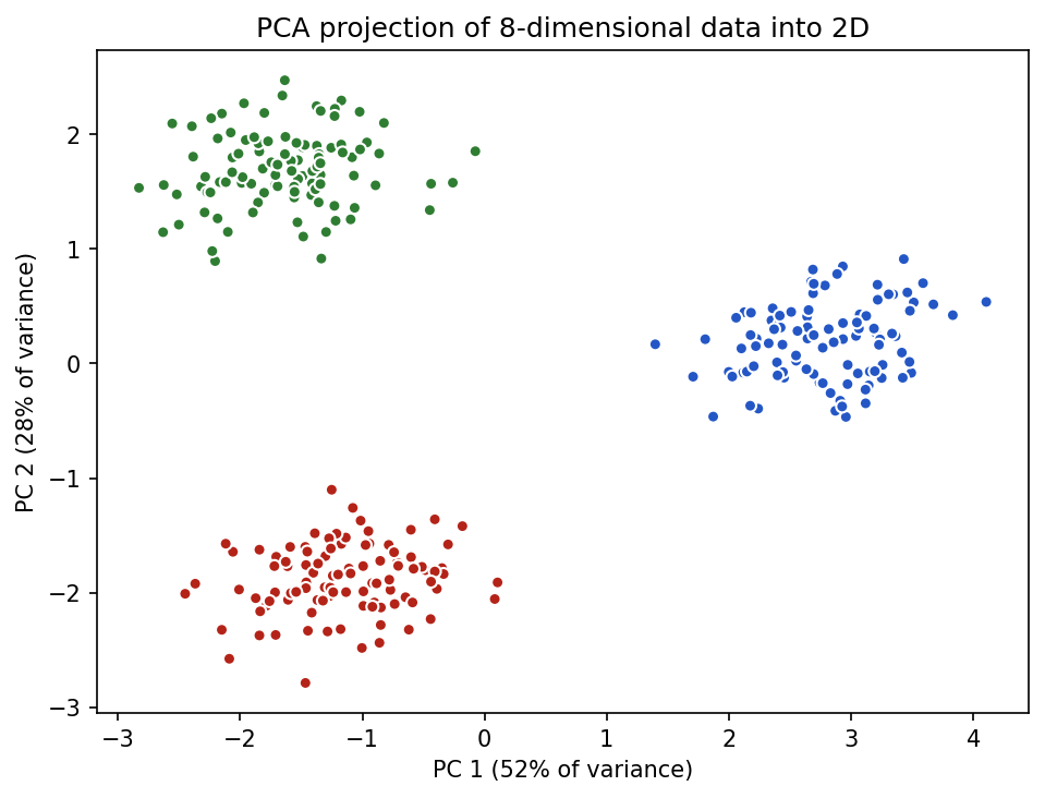
plt.title('PCA projection of 8-dimensional data into 2D')
plt.show()

PCA: keep the directions of greatest variance

Principal Component Analysis finds new axes (principal components) ordered by how much of the data's variance they capture. The first component is the single direction along which the data spreads the most; the second is the next-best direction at right angles to it, and so on. Keep the first few components and you keep most of the information in far fewer numbers.

PCA is linear, fast, and reversible-ish — a solid default for compression and de-noising.

from sklearn.decomposition import PCA
reduced = PCA(n_components=2).fit_transform(features)

t-SNE and UMAP: for visualization

t-SNE and UMAP are non-linear methods built mainly to visualize high-dimensional data in 2D. They try to keep points that were close together in the original space close in the plot, which makes clusters pop out. They are excellent for seeing structure (for example, whether weld images of different defect types form separate groups) but the axes have no simple meaning and distances between far-apart clusters are not reliable.

Autoencoders and latent spaces

An autoencoder is a neural network that squeezes input through a narrow middle layer and reconstructs it. That narrow middle — the latent space — is a learned, compressed representation. It is dimensionality reduction done by a network, and it can capture non-linear structure that PCA cannot.

Choosing a method

• Need a fast, general-purpose compression or de-noising step → PCA.
• Need to see clusters in 2D → t-SNE or UMAP (UMAP is usually faster).
• Working with images or complex data and have a network already → an autoencoder.